5 random variables as measurable functions and related results
A Course in Mathematical Statistics
... Random Variables and Their Distributions 53 3.1 3.2 3.3 3.4 3 .5* Chapter Some General Concepts 53 Discrete Random Variables (and Random Vectors) 55 Exercises 61 Continuous Random Variables (and ... Distribution 79 Exercises 82 Random Variables as Measurable Functions and Related Results 82 Exercises 84 Distribution Functions, Probability Densities, and Their Relationship 85 4.1 4.2 4.3 4.4* Chapter ... matching and the section on product probability spaces are also marked by an asterisk for the reason explained above In Chapter 3, the discussion of random variables as measurable functions and related...
Ngày tải lên: 09/06/2015, 15:11

independent and stationary sequences of random variables
... by the symbol E(X) I f X is a random vector with values in R" and distribution F, and is a Borel measurable function from R" to R, then (X) is a random variable, and E O (X) = J R" (x) F (dx) ... events), and P a measure on tR with P (Q) = For E E R, P (E) is called the probability of the event E A random variable X is a real-valued measurable function on (Q, a), and the measure F defined ... R, and let X be a random variable with E I X I < oo The conditional expectation of X relative to a1 is the random variable, denoted by E (X I 1), which is measurable with respect to tall and...
Ngày tải lên: 08/04/2014, 12:28

Báo cáo toán học: " A note on the almost sure limit theorem for self-normalized partial sums of random variables in the domain of attraction of the normal law" pptx
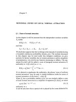
... Some ASCLT results for partial sums were obtained by Lacey and Philipp [4], Ibragimov and Lifshits [5] , Miao [6], Berkes and Cs´ ki [7], H¨ rmann [8], Wu [9, 10], and Ye and Wu [11] Huang and ... different character as CLT The difference between CLT and ASCLT lies in the weight in ASCLT The terminology of summation procedures (see, e.g., Chandrasekharan and Minakshisundaram [14, p 35] ) shows that ... (14) ( 15) (16) where dk and Dn are defined by (4) and f is a non-negative, bounded Lipschitz function Proof ¯ By the cental limit theorem for i.i.d random variables and VarS n ∼ nl(ηn ) as n →...
Ngày tải lên: 20/06/2014, 21:20

Báo cáo hóa học: "Research Article Recurring Mean Inequality of Random Variables" doc
... We define the random variable ζ, and assign P ζ λi ζβi /2 , i 1, , n Notice that λ1 and λn are the upper and lower bounds of the random variable ζ, so li and Li are the lower and upper bounds ... inequality of two random variables Theorem 1.6 Let ξ and η be bounded random variables If inf ξ > and inf η > 0, then Eξ ·Eη2 A ξ, η ≤ E2 ξη G ξ, η 1.6 Equality holds if and only if P ξ η a ... between stochastic inequalities and some classical mathematical inequalities,” Journal of Inequalities and Applications, vol 1, no 1, pp 85 98, 1997 M Wang, “The mean inequality of random variables, ”...
Ngày tải lên: 22/06/2014, 02:20

Independent And Stationary Sequences Of Random Variables ppt
... by the symbol E(X) I f X is a random vector with values in R" and distribution F, and is a Borel measurable function from R" to R, then (X) is a random variable, and E O (X) = J R" (x) F (dx) ... R, and let X be a random variable with E I X I < oo The conditional expectation of X relative to a1 is the random variable, denoted by E (X I 1), which is measurable with respect to tall and ... I) If Y and Z are random variables with E I YI < oc and E IZI < oo, and if Z is measurable with respect to a,, then with probability one, E(ZYI U1) = ZE(Y I UI) If a-algebras U 1, U satisfy...
Ngày tải lên: 27/06/2014, 03:20

Independent And Stationary Sequences Of Random Variables - Chapter 1 pptx
... by the symbol E(X) I f X is a random vector with values in R" and distribution F, and is a Borel measurable function from R" to R, then (X) is a random variable, and E O (X) = J R" (x) F (dx) ... R, and let X be a random variable with E I X I < oo The conditional expectation of X relative to a1 is the random variable, denoted by E (X I 1), which is measurable with respect to tall and ... I) If Y and Z are random variables with E I YI < oc and E IZI < oo, and if Z is measurable with respect to a,, then with probability one, E(ZYI U1) = ZE(Y I UI) If a-algebras U 1, U satisfy...
Ngày tải lên: 02/07/2014, 20:20

Independent And Stationary Sequences Of Random Variables - Chapter 2 ppt
... do-+0 as n-*co, proving (2 .5. 6) Lemma 2 .5. 2 The functions a (0) and b (o) of Lemma 2 .5. 1 have the properties (1) (2) the function a(o) is strictly increasing in [0, n], the function b (0) has exactly ... oo, 0] and has just one zero, and that simple, in (0, oo), and (2) for a > the function is non-zero in [0, oo] and has one simple zero in (- oo, 0) (4) Completion of the proof of Theorem 2 .5. 3 ... (A) and (B) with their oscillating integrands In this section we present a series of asymptotic formulae due to Linnik [99], Skorokhod [174] Bergstrom [16] and Pollard [1 35] The special case...
Ngày tải lên: 02/07/2014, 20:20
Independent And Stationary Sequences Of Random Variables - Chapter 4 ppt
... , b2, be independent and identically distributed random variables taking only the values and 1, with respective probabilities b and a Bernstein's inequality (cf § 7 .5) shows that n) ()a m b ... the local limit theorems for the case of normal convergence In this section we assume that the common distribution of the random variables X; has zero mean and finite variance o We write (x) ... of independent random variables with distribution F, and denote as before by Fn (x) the distribution function of the normalised sum Z,, = (X + X2 + + Xn - An)/ B,, Then Fn has a similar decomposition...
Ngày tải lên: 02/07/2014, 20:20
Independent And Stationary Sequences Of Random Variables - Chapter 5 pot
... (2) 1
Ngày tải lên: 02/07/2014, 20:20
Independent And Stationary Sequences Of Random Variables - Chapter 6 pptx
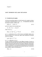
... (6 7) We remark that the asymptotic formula (6.1 6) can be very useful, and is often much easier to compute than the exact expression (6 5) Suppose that the random variables X; introduced at ... situation is analogous to the classical case, in which a whole class of distributions is attracted to the same stable law It is however in sharp contrast to the case a=-!, in which the whole function ... INTRODUCTION AND EXAMPLES 55 when both n and x are large Such problems constitute the theory of large deviations Since the...
Ngày tải lên: 02/07/2014, 20:20
Independent And Stationary Sequences Of Random Variables - Chapter 7 potx
... 161-1 65) We assume that the independent random variables X1 , X2 , satisfy E (Xl) = a1 , V (Xl) _ #j , (7 .5. 1) and write ZI =XI -a1 , Bn=/31+fl2+ +/3n, Sn = Z I +Z2+ +Zn Theorem 5. 1 ... 2=6 , 73 = P3, Y4=°4 - 354 , Y5 = 5 - 1O° 35 , etc are the cumulants of Xi and ° j are the moments of Xj Turning now to (7.2.6), we assume that x = o (n4), so that T >0 as The saddle point equation ... has an analytic continuation to the strip IRe z( < a, which has a power series expansion about z = convergent in tzI < 2a-a The integrand in (7.2.4) has the form M (z)" exp (- cn zx) (7.2 .5) ...
Ngày tải lên: 02/07/2014, 20:20
Independent And Stationary Sequences Of Random Variables - Chapter 8 pps
... introduction of auxiliary random variables Since E (exp a JXX j) < oo , we may write, for Jhj
Ngày tải lên: 02/07/2014, 20:20
Independent And Stationary Sequences Of Random Variables - Chapter 9 ppsx
... exp ( - c1 n 2a p (n)") 79 (9 5) Since a < Z, /3 < and (9 2 .5) contradicts (9.2.4) The case of (9.2 3) is treated similarly Theorem 2 For random variables of class (d) the condition (9.2 1) ... a') , (9 .5 15) or, taking into account (9 5. 13) and (9 5. 14), n_° 0f p n (x) = 2n nl exp(-2nt ) Z r=,,,+3 X' t' exp(-i0In° (9 .5. 16) where R = B exp (-c4 711n "')+B exp(-E n a'), (9 .5 17) and E3 ... (9 .5 1) DERIVATION OF THE BASIC INTEGRAL Now Re nK (t) < for I tl m and writing ,/, tr = r=so+3 Yr r -, , E r Kso+3 we have, from (9 4 .5) , p© < n - 41, 1 85 (9 14) (x) = n J -27r (9 2) and...
Ngày tải lên: 02/07/2014, 20:20
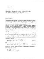
Independent And Stationary Sequences Of Random Variables - Chapter 10 potx
... ), (10 .5. 2) where C becomes arbitrarily large for large C If < x < n§`/p (n) and s satisfies (10.1 6), then nr3 AEC 1I (i) = ni3 2ts] (i)+Bn_E ( 10 .5 3) Substituting (10 5. 1), (10 .5. 2) and (10 ... relations like (10 1.2) and (10.1 3) imply local normal convergence In the last chapter the zones of local normal convergence were characterised, so that we may take this case as having been dealt ... proof of the theorem for < x < na/ p (n) The case -n"/p(n)
Ngày tải lên: 02/07/2014, 20:20
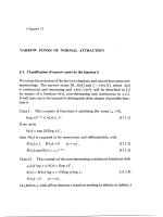
Independent And Stationary Sequences Of Random Variables - Chapter 11 doc
... special case of monomial zones We now proceed to the general case „ 15 The general case of narrow zones We now follow the argument of „„ 11-14 to prove Theorem 11 2.2 Let XX be random variables ... < It is natural to assume h to be monotonic and differentiable, so that H is also If we also assume that h' is monotonic, this leads to (11 2) and, in view of the left-hand inequality of (11 ... For h in Class III, we take A(n)= {log n} , , (11 4) thus delimiting "very narrow" zones Theorem 11 2 .5 For h (x) in Class III and A (n) = {log n} the statements ofTheorems 11 2.1 and 11 2.2...
Ngày tải lên: 02/07/2014, 20:20

Independent And Stationary Sequences Of Random Variables - Chapter 12 ppsx
... (n) < n P3 (n) ICI (12 .5. 6) ( 12 .5. 7) Now consider the function W" (u) _fu f" (~) d~ , (12 .5. 8) and write 2T={~
Ngày tải lên: 02/07/2014, 20:20
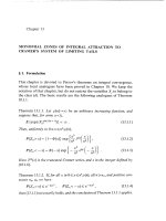
Independent And Stationary Sequences Of Random Variables - Chapter 13 pdf
... 2.2) Zn = Sn/6n- , and a modified random variable Z n = Zn + Yn /6n ( 13 3) , where Yn is a random variable, independent of the Xj , and having a normal distribution with mean and variance n " ... distribution functions of Z n and n will be denoted by Fn (x) and Fn (x) respectively, and their characteristic functions by fn (t) and fn(t), so that n2"-1 t fn (t) = fn (t) eXp - X62 (13 5) 246 ... that t -).O as n co Form the equation dz {K (13 2.12) N (z)-zta} = For sufficiently small t, this equation has a unique real root z o with the same sign as t and tending to zero as t >0 In...
Ngày tải lên: 02/07/2014, 20:20
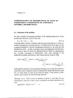
Independent And Stationary Sequences Of Random Variables - Chapter 14 docx
... t>,0 and downwards for t,, (since the variance exists), the A, are constants, with A a > 0, and s>0 The class of ... dx - nP(X1 > yun ) - nAa/o-a ya n 2a (14 .5. 4) In particular, taking y = x n , nAa/faxan2a = BE n -2' 3+E , ( 14 .5. 5) and so, combining (14 3) and (14 .5. 4), f n (x) dx = P (Z,, > x) _ "o p X =...
Ngày tải lên: 02/07/2014, 20:20
Independent And Stationary Sequences Of Random Variables - Chapter 15 pptx
... , ( 15. 4.14) since we have assumed that n > 15 PROOF OF THEOREM 15 1 283 Consequently IF2 -F3 ) < C n +C 13 n - I < C 14 n - - ,, f ( 15. 4. 15) and combining ( 15 9), ( 15. 4.11) and ( 15 4. 15) ... we shall assume that the distribution function F(x) of the variables X3 is continuous and strictly increasing As in ± 2, X1 = F -1 (~r), where (~;) is a sequence of independent random variables, ... 15 ( 15. 4 10) Without loss of generality we can take n > ; then the right-hand side of ( 15. 4.10) does not exceed C4 C7k (1- Zn ) < 2C4 C 7k This is the analogue of ( 15. 4 .5) in (II), and as...
Ngày tải lên: 02/07/2014, 20:20
Independent And Stationary Sequences Of Random Variables - Chapter 16 ppsx
... probability Since each random variable ~, measurable with respect to M, is the limit as n ' co with probability 1, of the random variables _ j ~n k=-cc k nx k -C n +1 n there exists one and only one transformation ... of stationary processes Xt , and every stationary process is so generated To prove this, associate with Tt a transformation Ti on the class of random variables measurable with respect to fit, ... these assertions is left to the reader THEORY OF STATIONARY PROCESSES : SOME RESULTS 286 Chap 16 ± Stationary processes and the associated measure-preserving transformations With each random...
Ngày tải lên: 02/07/2014, 20:20