10 ecologically based planning and design techniques
A textbook of Computer Based Numerical and Statiscal Techniques part 10 ppt
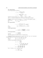
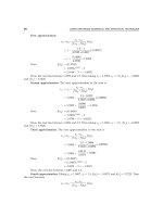
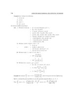
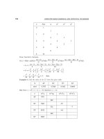
... x∞ ) + f ′′( x∞ )Ek − ≈ Ek f ′( x∞ ) + f ′′( x∞ )( Ek + Ek − ) . (10) .(11) .(12) 82 COMPUTER BASED NUMERICAL AND STATISTICAL TECHNIQUES f ′′( x∞ )(Ek + Ek −1 ) is negligible compared to f ′( ... x1 = and f(x0) = 20, f(x1) = – 1, then by Secant method the next approximation is given by x1 − x0 x = x1 – f(x1) f ( x1 ) − f ( x0 ) 84 COMPUTER BASED NUMERICAL AND STATISTICAL TECHNIQUES ... î + å n ) f ( î + å n ) − f ( î + å n −1 ) .(2) On expanding f (î + å n ) and f (î + å n−1) in Taylor’s series about the point î in (2), and using f (ξ) = 0, we obtain εn + 1 (εn − εn −1 ) εn...
Ngày tải lên: 04/07/2014, 15:20

LTCI PLANNING AND SALES TECHNIQUES FACT FINDERS potx
... (remember, not individual and the retirement plan • Expand the discussion based on the discussion created by the above statement Do not talk about LTCI Establish the connection based on your strength ... love you and want to make sure you are safe The plan I want to put together recognizes that one or more may be available It can allow them to provide the care you need and want longer and better ... and assisted care Even if you decide you want to go to a nursing home when you first need long term care you will have to transfer most of your assets including qualified funds and low cost based...
Ngày tải lên: 07/03/2014, 14:20

A textbook of Computer Based Numerical and Statiscal Techniques part 62 docx
... h) Step End loop i Step 10 Result = sum * h/3 Step 11 Step 12 Print output End of the program and start of section func 599 600 COMPUTER BASED NUMERICAL AND STATISTICAL TECHNIQUES Step 13 temp ... When x = 9.0, y = 810. 00 Press enter to exit 13.28 ALGORITHM FOR TRAPEZOIDAL RULE Step Start of the program for numerical integration Step Input the upper and lower limits a and b Step Step Obtain ... value of the function = 1 .103 846 13.30 ALGORITHM FOR SIMPSON’S 1/3 RULE Step Step Start of the program for numerical integration Input the upper and lower limits a and b Step Obtain the number...
Ngày tải lên: 04/07/2014, 15:20

A textbook of Computer Based Numerical and Statiscal Techniques part 1 ppt
... 4835/24, Ansari Road, Daryaganj, New Delhi - 1100 02 Visit us at www.newagepublishers.com Preface The present book ‘Computer Based Numerical and Statistical Techniques is primarily written according ... concepts, definitions and large number of examples in the best possible way have been discussed in detail and lucid manner so that the students should feel no difficulty to understand the subject A ... subject A unique feature of this book is to provide with an algorithm and computer program in Clanguage to understand the steps and methodology used in writing the program Thorough care has been...
Ngày tải lên: 04/07/2014, 15:20
A textbook of Computer Based Numerical and Statiscal Techniques part 2 ppsx
... it is to COMPUTER BASED NUMERICAL AND STATISTICAL TECHNIQUES be cut-off to a manageable size such as 0.29, 0.286, 0.2857, etc The process of cutting off super-flouts digits and retaining as many ... 7326853000 becomes 7327 × 106 1.3 ERRORS Error = True value – Approximate value A computer has a finite word length and so only a fixed number of digits are stored and used during computation ... machine dependent and is called machine epsilon After the computation is over, the result in the machine form (with base b) is again converted to decimal form understandable to the users and some more...
Ngày tải lên: 04/07/2014, 15:20

A textbook of Computer Based Numerical and Statiscal Techniques part 3 ppsx
... equation X2 – 2X + log10 = are given by, X = δX Therefore, = ± − log10 2 = ± − log 10 δ(log 2) < 0.5 × 10 4 − log δ(log 2) < × 0.5 × 10 4 (1 − log 2)1/2 < 0.83604 × 10 −4 or ≈ 8.3604 × 10 5 Example 21 ... ≤ x + x + + x n 10 COMPUTER BASED NUMERICAL AND STATISTICAL TECHNIQUES 0.0005 0.0005 + = 0.0002501 3.724 4.312 Therefore, Relative Error, Er = (Because Error = 1 × 10 − n = × 10 −3 = 0.0005) ... 5V δu = ∂u δV = (12V − 5)δV ∂V 14 COMPUTER BASED NUMERICAL AND STATISTICAL TECHNIQUES 12V − ∂u δV × 100 100 = 2V − 5V u (12 − 5) × 0.05 × 100 = − × = −11.667% (2 − 5) Hence maximum...
Ngày tải lên: 04/07/2014, 15:20
A textbook of Computer Based Numerical and Statiscal Techniques part 4 ppt
... − b − ac 2a a = = 0 .100 0 × 101 b = 400 = 0.4000 × 10³ c = 1= 0 .100 0 × 101 b2 – 4ac = 0.1600 × 10⁶ – 0.4000 × 101 = 0.1600 × 10⁶ (To four-digit accuracy) b − 4ac = 0.4000 × 10 On substituting these ... as x = 2c b + b − 4ac 20 COMPUTER BASED NUMERICAL AND STATISTICAL TECHNIQUES x = 0.2000 × 101 0.4000 × 10³ + 0.4000 × 10³ x = or 0.2000 × 101 = 0.0025 0.8000 × 10 This is the exact root of the ... δa = 0.1 a× 100 δb = ⇒ δb = 0.2 b× 100 (1) 19 ERRORS AND FLOATING POINT ∂A −a ∂A = = and 2 ∂b b b − a ∂a b −a Substituting these values in equation (1), we have δA < 0.00135 + 0.0 0100 < 0.00235...
Ngày tải lên: 04/07/2014, 15:20

A textbook of Computer Based Numerical and Statiscal Techniques part 5 ppsx
... x2 – 100 0x + 25 = Sol Given that, x2 – 100 0x + 25 = x= ⇒ Now 100 0 ± 106 − 102 106 = 0.000e7 and 102 = 0 .100 0e3 Therefore 106 – 102 = 0 .100 0e7 ⇒ Hence roots are: 0 .100 0e + 0 .100 0e 0 .100 0e ... 0.36143447 × 10 gives 0.0001 1101 × 107 On shifting the fractional part three places to the left we have 0.1 1101 × 104 which is obviously a floating-point number Also 0.0001 1101 × 107 is a floating-point ... 0 .100 0e7 ⇒ Hence roots are: 0 .100 0e + 0 .100 0e 0 .100 0e − 0 .100 0e and 2 106 − 10 = 0 .100 0e which are 0 .100 0e4 and 0.0000e4 respectively One of the roots becomes zero due to...
Ngày tải lên: 04/07/2014, 15:20

A textbook of Computer Based Numerical and Statiscal Techniques part 6 pptx
... equation x log 10 x = 1.2 by Bisection Method Sol Let f ( x) = x log10 x − 1.2 = So that f (1) = log10 − 1.2 = −1.2 < f (2) = 2log10 − 1.2 = 0.602 − 1.2 and = − 0.598 < f (3) = 3log10 − 1.2 and = 3(0.4771) ... −1 , which is negative Thus f(0.5) is negative and f(1) is positive Then the root lies between 0.5 and 40 COMPUTER BASED NUMERICAL AND STATISTICAL TECHNIQUES Second approximation: The second approximation ... ALGEBRAIC AND TRANSCENDENTAL EQUATION Here ei and ei + are the errors in ith and (i + 1)th iterations respectively Comparing the above equation with lim i →∞ ei +1 e k i ≤A We get k = and A = 0.5...
Ngày tải lên: 04/07/2014, 15:20
A textbook of Computer Based Numerical and Statiscal Techniques part 7 potx
... (2) f(3) = (3)3 – 9(3) + = 52 COMPUTER BASED NUMERICAL AND STATISTICAL TECHNIQUES Since f(2) and f(3) are of opposite signs, therefore the root lies between and 3, so taking x0 = 2, x1 = 3, f(x0) ... So that f(2) = (2)3 – 2(2) – = – 50 COMPUTER BASED NUMERICAL AND STATISTICAL TECHNIQUES f(3) = (3)3 – 2(3) – = 16 Therefore, a root lies between and First approximation: Therefore taking x0 = ... COMPUTER BASED NUMERICAL AND STATISTICAL TECHNIQUES Example Find a real root of the equation f(x) = x3 – x2 – = by Regula-Falsi method Sol Let Then, f(x) = x3 – x2 – = f(0) = – 2, f(1) = – and f(2)...
Ngày tải lên: 04/07/2014, 15:20
A textbook of Computer Based Numerical and Statiscal Techniques part 8 doc
... = – 0.2475 and f(x1) = 2.6137 Then the root is x = x0 − x1 − x0 f ( x0 ) f ( x1 ) − f ( x0 ) 58 COMPUTER BASED NUMERICAL AND STATISTICAL TECHNIQUES = 3. 6106 – = 3. 6106 + Now, − 3. 6106 (−0.2475 ... (3. 6106 )2 – loge (3. 6106 ) – 12 13.0364 – 13.2839 = – 0.2475 The root will lies between 3. 6106 and Therefore for next =3+ Now, f(x2) = = = Second approximation: approximation, taking x0 = 3. 6106 , ... = f(3) = 32 – loge – 12 = – 4.0986 and f(4) = 42 – loge – 12 and 2.6137 Therefore, f(3) and f(4) are of opposite signs Therefore, a real root lies between and For the approximation to the root,...
Ngày tải lên: 04/07/2014, 15:20

A textbook of Computer Based Numerical and Statiscal Techniques part 9 docx
... x0 + 10 3x0 + x0 + 10 2((1.2 ) + (1.2) + 10) = or ) (1.2) + (1.2) + 10 26.336 19.12 x1 = 1.3774059 Second approximation: x2 = ( 2 x1 + x1 + 10 3x1 ) + x1 + 10 (1.3774059) + (1.3774059 ) + 10 = ... xn+1 = f ( xn ) f ′ ( xn ) xn + 2xn + 10 xn − 20 3xn + 4xn + 10 ( 2 xn + xn + 10 ) .(1) + xn + 10 f(1) = – < and f(2) = 16 > 3xn Therefore root lies between and Let x0 = 1.2 be the initial approximation ... 1.3774059 + 10 x2 = 1.3688295 = 29.0 2105 2 2.201364 71 ALGEBRAIC AND TRANSCENDENTAL EQUATION Third approximation: x3 = or x3 2( x2 + x2 + 10) 3x2 + 4x2 + 10 2(1.3688295) + (1.3688295) + 10 28.876924...
Ngày tải lên: 04/07/2014, 15:20
A textbook of Computer Based Numerical and Statiscal Techniques part 11 pdf
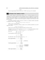
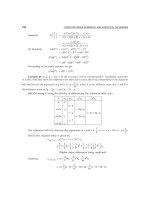
... 2, 3, 4, ∂q ∂q .(11) 94 COMPUTER BASED NUMERICAL AND STATISTICAL TECHNIQUES ∂br +1 ∂br =0 = ∂q ∂p Now, an equation (10) and (11) shows that Now set, Thus from (10) ∂br ∂p – − = Cr–1 so that – ... can now be repeated with three approximations as 1.780776, 1.837867, and 1.839284 90 COMPUTER BASED NUMERICAL AND STATISTICAL TECHNIQUES Let Then xi − = 1.780776, xi −1 = 1.837867, xi = 1.839284 ... quadratic factors that are the products of the pairs of 92 COMPUTER BASED NUMERICAL AND STATISTICAL TECHNIQUES complex roots, and then complex arithmetic can be avoided because such quadratic factors...
Ngày tải lên: 04/07/2014, 15:20
A textbook of Computer Based Numerical and Statiscal Techniques part 12 pdf
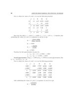
... 10. 480733 After substituting the values of bi and Ci in equations (1) and (2), we get ∆p = 0.018582 ∆q = – 0.0002186 100 COMPUTER BASED NUMERICAL AND STATISTICAL TECHNIQUES Therefore the third approximation ... −1.151474 8.262097 0. 2100 54 0.441998 3.848526 10. 379674 43.624369 92.859594 3.848526 −7.306426 bi 3.848526 −7.306426 Ci −7.306426 −19.705 810 −82.820859 2.697052 11.335345 24.128613 10. 480733 After ... b2 = 0, where bi are given by the same procedure, when p and q are of required accuracy 98 COMPUTER BASED NUMERICAL AND STATISTICAL TECHNIQUES a1 1.9882 −6 18 −24 16 1.9882 −7.97626 15.95299...
Ngày tải lên: 04/07/2014, 15:20
A textbook of Computer Based Numerical and Statiscal Techniques part 13 doc
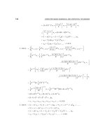
... 9397 −334 −69 25 9063 −403 30 8660 From the table, ∆2y10,∆4y5 is as ∆2y10 = –73 and ∆4y5 = –1 108 COMPUTER BASED NUMERICAL AND STATISTICAL TECHNIQUES Example Find f(6) given that f(0) = –3, f(1) ... 10 20 30 40 50 y 1.3 010 1.4771 1.6021 1.6990 and find the values of ∇ log 40 and ∇ log 50 Sol For the given data, backward difference table as: x 10 ∇y y ∇2 y ∇3y ∇4 y 0.3 010 −0.1249 20 1.3 010 ... + 10 2f (–1) + 10 3f(–1) = [ f(–1) + ∆f(–1)] +4[∆f(–1)+ ∆2f(–1)] + 6∆2 f(–1) + 10 3f(–1) = [ f (−1) + ∆f (−1)] + ∆[ f (−1) + ∆f (−1)] + ∆ f ( −1) + 10 ∆ f (−1) = f (0) + ∆f (0) + ∆ f ( −1) + 10...
Ngày tải lên: 04/07/2014, 15:20
A textbook of Computer Based Numerical and Statiscal Techniques part 14 ppsx
... 2 2 2 1 1 = f (x + ) g(x – ) – f(x – ) g(x + ) 2 2 = 124 COMPUTER BASED NUMERICAL AND STATISTICAL TECHNIQUES Therefore right hand side as 1 1 f (x + ) g (x − ) − f (x − ) g (x + ) 2 2 = 1 g( x ... g(x) g(x − )g(x + ) 2 Here, interval of differencing being unity 120 COMPUTER BASED NUMERICAL AND STATISTICAL TECHNIQUES (b) ∇ = h2 D2 – h3 D3 + 4 – h D 12 (c) ∇ – ∆ = – ∇ ∆ δ2 (d) + ... 2 2 = ( ∆y x ) + Hence, µδ = 1 (∇ y x ) = 2 (∆ + ∇) ( ∆ + ∇ ) yx 122 COMPUTER BASED NUMERICAL AND STATISTICAL TECHNIQUES Example 22 Evaluate: ∆n [sin (ax + b)] Sol We know ∆f (x) = f(x + h)...
Ngày tải lên: 04/07/2014, 15:20
A textbook of Computer Based Numerical and Statiscal Techniques part 15 doc
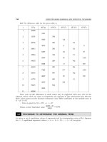
... 200, u4 = 100 , u5 = Find the value of ∆ 5u0 Sol We know ∆ = E – 1, therefore, ∆ u0 = (E –1)5u0 = (E5 – 5E4 + 10E3 – 10E2 + 5E – 1)u0 = u5 – 5u4 + 10u3 – 10u2 + 5u1 – u0 = – 500 + 2000 – 810 + 60 ... in following entries and correct it 1.203, 1.424, 1.681, 1.992, 2.379, 2.848, 3.429, 4.136 Sol Difference table for given data is as follows: 103 y 103 ∆y 103 ∆ y 103 ∆ y 10 ∆ y 1203 221 1424 ... 130321 40 48 408 21455 104 976 −20 352 2706 65540 160000 28 134 COMPUTER BASED NUMERICAL AND STATISTICAL TECHNIQUES From this table we have the third differences are quite iregular and the irregularity...
Ngày tải lên: 04/07/2014, 15:20
A textbook of Computer Based Numerical and Statiscal Techniques part 16 ppsx
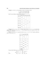
... 350 ? 430 [Ans f(1964) = 306 f(1966 = 390)] Given, log 100 = 2, log 101 = 2.0043, log 103 = 2.0128, log 104 = 2.0170 find log 102 [Ans log 102 = 2.0086] Estimate the missing term in the following: ... and 20f (5) + 6f(3) = 2662 i.e., f(5) + f(3) = 152 and 10f(5) + 3f(3) = 1331 On solving these two, we get f(3) = 27 and f(5) = 125 Example 10 Assuming that the following values of y belong to ... get 81 − f (3) + × − × + = .(1) 138 COMPUTER BASED NUMERICAL AND STATISTICAL TECHNIQUES i.e., 4f(3) = 124 i.e., f(3) = 31 (function values are 3n type and this is not a polynomial) Example Find...
Ngày tải lên: 04/07/2014, 15:20
A textbook of Computer Based Numerical and Statiscal Techniques part 17 ppsx
... function f ( x) by x Then the remainder will be 10 and the quotient will be 2x − 3x + ∴ D = 10 152 COMPUTER BASED NUMERICAL AND STATISTICAL TECHNIQUES Now divide the quotient by (x – 1) i.e., ... multiply –3 by and by and add them to get the sum –1 which is to be written below The remainder 10 is the value of D Add the terms of corresponding columns of (a) and get 2, –1 and of (b) Now ... COMPUTER BASED NUMERICAL AND STATISTICAL TECHNIQUES Example 13 Prove that if m is a positive integer then ( x + 1)(m) m! = x(m) x(m−1) + m! (m − 1)! Sol To prove this we start from R.H.S and use...
Ngày tải lên: 04/07/2014, 15:20
A textbook of Computer Based Numerical and Statiscal Techniques part 19 pptx
... 10 [Ans 2x3-7x2+6x+1] Find the number of men getting wages between Rs 10 and Rs.15 from following table: Wages (in Rs.) − 10 10 − 20 20 − 30 30 − 40 Frequency 30 35 42 [Ans 15] 172 COMPUTER BASED ... the arithmetic mean of q and r and B is arithmetic between the arguments at q and r is A + 24 mean of 3q – 2p – s and 3r – 2s – p Sol Given A is the arithmetic mean of q and r q+r q + r = 2A ⇒ ... 0.40 ∇3 ∇4 0 .100 3 0.0508 0.15 0.1511 0.0008 0.0516 0.20 0.2027 0.0002 0.0 010 0.0526 0.25 0.2553 0.30 0.3093 0.0004 0.0014 0.0540 0.0002 174 COMPUTER BASED NUMERICAL AND STATISTICAL TECHNIQUES (a)...
Ngày tải lên: 04/07/2014, 15:20
Bạn có muốn tìm thêm với từ khóa:
- chapter 10 planning and cabling networks answers
- ccna chapter 10 planning and cabling networks
- planning and cabling networks chapter 10
- robust nonlinear control design statespace and lyapunov techniques pdf
- ccna 1 chapter 10 planning and cabling networks
- robust nonlinear control design statespace and lyapunov techniques