Proakis J (2002) Communication Systems Engineering - Solutions Manual (299s) Episode 10 pot

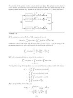
... figure. 0000 0001 0101 0100 1100 1101 101 0 0 110 0 010 0011 100 1 100 0 101 1 0111 1111 1 110 1 1 1 1 1 1 1 1 1 1 1 1 2 2 1 21 2 2 1 2 1 Problem 7.46 1) Consider the QAM constellation of Fig. P-7.46. Using ... points are connected with solid or dashed lines. 0000 0001 0011 0 010 0 110 0111 0101 0100 1100 1101 1111 1 110 1 010 1011 100 0 100 1 196 ... is A =  44.9...

Ngày tải lên: 12/08/2014, 16:21

... 100 1101 100 1011 100 1000 c 9 0 1101 10 1 1101 10 0 0101 10 0100 110 0111 110 0 1100 10 0 1101 00 0 1101 11 c 10 0101 100 1101 100 000 1100 011 1100 0100 100 0101 000 0101 110 0101 101 c 11 00 1101 0 101 1 010 01 1101 0 00 0101 0 ... 0001 110 c 6 1100 101 0100 101 100 0101 1 1101 01 1101 101 1100 001 1100 111 1100 100 c 7 101 0011 0 0100 11 1 1100 11 100 0011 101 1011 101 01...

Ngày tải lên: 12/08/2014, 16:21

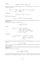
... then x n = 1 T  T 2 − T 2 x(t)e j2 π n T t dt = 1 T  T 2 − T 2 e j2 π n T t dt + 1 T  T 4 − T 4 e j2 π n T t dt = j 2πn e j2 π n T t     T 2 − T 2 + j 2πn e j2 π n T t     T 4 − T 4 = j 2πn  e j n − e j n + e j n 2 − ... =  n  i=1 α 2 i  1 2 ,B=  n  i=1 β 2 i  1 2 8 c) X(f)=  ∞ −∞ x(t)e j2 πft dt =  0 −1 (t +1)e j2 πft dt +  1 0 (t − 1)e j2 πft dt =  j...

Ngày tải lên: 12/08/2014, 16:21

... +8× 10 5 +10 3 )  −25  1 j δ(f − 8 × 10 5 +10 3 ) − 1 j δ(f +8× 10 5 − 10 3 )  +125  δ(f − 8 × 10 5 − 2 × 10 3 )+δ(f +8× 10 5 +2× 10 3 )  +125  δ(f − 8 × 10 5 − 2 × 10 3 )+δ(f +8× 10 5 +2× ... 10 5 +2× 10 3 )  = 50[δ(f − 8 × 10 5 )+δ(f +8× 10 5 )] +25  δ(f − 8 × 10 5 − 10 3 )e j π 2 + δ(f +8× 10 5 +10 3 )e j π 2  +25  δ(f − 8 × 10...

Ngày tải lên: 12/08/2014, 16:21

... Note that J 0 (1.5) = .5118, J 1 (1.5) = .5579 and J 2 (1.5) = .2321. 63 ✲✛ ✻ ✻ ✻ ✻ ✻ ✻ ✻ ✻ ✻ ✛ ✲ ✻ ✻ ✻ ✻ ✻ AJ 4 (3) 2 AJ 2 (3) 2 8 10 3 10 6 f Hz 5 10 3 AJ 2 (1.5) 2 AJ 1 (1.5) 2 f Hz 10 6 5) ... k. Index k J k (2) Frequency Hz Amplitude 10 0J k (2) Power P f c +kf m 0 .2239 10 8 22.39 250.63 1 .5767 10 8 +10 4 57.67 1663.1 2 .3528 10 8 +2× 10 4 35.28 622.46 3 .128...

Ngày tải lên: 12/08/2014, 16:21

... 1.59 × 10 −1 1.587 × 10 −1 1.5 6.68 10 −2 6.685 × 10 −2 2. 2.28 × 10 −2 2.276 × 10 −2 2.5 6.21 10 −3 6.214 × 10 −3 3. 1.35 × 10 −3 1.351 × 10 −3 3.5 2.33 10 −4 2.328 × 10 −4 4. 3.17 × 10 −5 3.171 ... 10 −5 3.171 × 10 −5 4.5 3.40 10 −6 3.404 × 10 −6 5. 2.87 × 10 −7 2.874 × 10 −7 Problem 4.25 The n-dimensional joint Gaussian distribution is f X (x)= 1  (2π) n...

Ngày tải lên: 12/08/2014, 16:21

... ,y n )= J  j= 1 f X(t 1 ), ,X(t n ) (x 1 , ,x n ) |J( x j 1 , ,x j n )| where J is the number of solutions to the system y 1 = Q(x 1 ),y 2 = Q(x 2 ), ···,y n = Q(x n ) and J( x j 1 , ,x j n ) is the Jacobian ... Q( a 13 √ 10 )=0.0431 p(ˆx 5 )=p(ˆx 12 )=Q( a 11 √ 10 ) − Q( a 12 √ 10 )=0.0674 p(ˆx 6 )=p(ˆx 11 )=Q( a 10 √ 10 ) − Q( a 11 √ 10 )=0.0940 p(ˆx 7 )=p(ˆx...

Ngày tải lên: 12/08/2014, 16:21

... to the dynamic range of the input signal for E[ ˘ X 2 ] > 1. -5 0 0 50 100 150 200 -1 00 -8 0 -6 0 -4 0 -2 0 0 20 40 60 80 100 mu-law uniform E[X^2] db SQNR (db) Problem 6.58 The optimal compressor ... g(1) = 1. Since the resulting distortion is (see Equation 6.6.17) -1 -0 .8 -0 .6 -0 .4 -0 .2 0 0.2 0.4 0.6 0.8 1 -1 -0 .8 -0 .6 -0 .4 -0 ....

Ngày tải lên: 12/08/2014, 16:21

... transition matrix of the (2,7) runlength-limited code is the 8 × 8 matrix D =               0100 0000 0 0100 000 100 10000 100 0100 0 100 0 0100 100 00 010 10000001 100 00000               Problem ... =          00 0100 100 100 0101 00 0 0101 0 0 0100 1 0 0100 0          236 Problem 8.32 The state transition matrix of the (0,1) runlength-...

Ngày tải lên: 12/08/2014, 16:21

... sequences of length 3 and the corresponding output of the detector. -1 -1 -1 -4 -1 -1 1 -2 -1 1 -1 0 -1 11 2 1-1 -1 -2 1-1 1 0 1 1-1 2 111 4 As it is observed there are 5 possible output levels b m , ... to d E =2 2 +4 2 +2 2 =24 ✉ ✉ ✉ ✉✉ ✉ ✉ ✉✉ ✉ ✉ ✉✉ ✉ ✉ ✉     ✒ ✲✲ ❍ ❍ ❍ ❍ ❍❥ ✟ ✟ ✟ ✟ ✟✯ ✲     ✒ ✟ ✟ ✟ ✟ ✟✯ ❅ ❅ ❅ ❅ ❅❘ ❍ ❍ ❍ ❍ ❍❥ ❍ ❍ ❍ ❍ ❍❥...

Ngày tải lên: 12/08/2014, 16:21