Proakis J (2002) Communication Systems Engineering - Solutions Manual (299s) Episode 5 docx

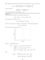
... +2Y>1) = 3 7 x 2 + 6 7 x + 3 7 80 + b2= 356 563782d+00, b3=1.781477937d+00, + b4 =-1 .821 255 978d+00, b5=1.330274429d+00) C- pi=4.*atan(1.) C-INPUT PRINT*, ’Enter -x-’ READ*, x C- t=1./(1.+p*x) a=b1*t + b2*t**2. ... 1 .59 × 10 −1 1 .58 7 × 10 −1 1 .5 6.68 ×10 −2 6.6 85 × 10 −2 2. 2.28 × 10 −2 2.276 × 10 −2 2 .5 6.21 ×10 −3 6.214 × 10 −3 3. 1. 35 × 10 −3 1. 351 × 10 −3 3 .5 2.33 ×10...

Ngày tải lên: 12/08/2014, 16:21

... then x n = 1 T  T 2 − T 2 x(t)e j2 π n T t dt = 1 T  T 2 − T 2 e j2 π n T t dt + 1 T  T 4 − T 4 e j2 π n T t dt = j 2πn e j2 π n T t     T 2 − T 2 + j 2πn e j2 π n T t     T 4 − T 4 = j 2πn  e j n − e j n + e j n 2 − ... frequency content. 13 SOLUTIONS MANUAL Communication Systems Engineering Second Edition John G. Proakis Masoud Salehi Prepared by Evang...

Ngày tải lên: 12/08/2014, 16:21

... that J 0 (1 .5) = .51 18, J 1 (1 .5) = .55 79 and J 2 (1 .5) = .2321. 63 ✲✛ ✻ ✻ ✻ ✻ ✻ ✻ ✻ ✻ ✻ ✛ ✲ ✻ ✻ ✻ ✻ ✻ AJ 4 (3) 2 AJ 2 (3) 2 8×10 3 10 6 f Hz 5 10 3 AJ 2 (1 .5) 2 AJ 1 (1 .5) 2 f Hz 10 6 5) If ... expansion c n = 1 T m  T m 0 e jm(t) e j2 πnf m t dt = 1 T m  T m 2 0 e j e j2 πnf m t dt + 1 T m  T m T m 2 e j e j2 πnf m t dt = − e j T m j2 πnf m e j2 πnf m t   ...

Ngày tải lên: 12/08/2014, 16:21

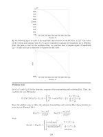
... ,y n )= J  j= 1 f X(t 1 ), ,X(t n ) (x 1 , ,x n ) |J( x j 1 , ,x j n )| where J is the number of solutions to the system y 1 = Q(x 1 ),y 2 = Q(x 2 ), ···,y n = Q(x n ) and J( x j 1 , ,x j n ) is the Jacobian ... ln(6)−ln( √ 6)+1/2=1.79 25 bits /source output. A plot of the lower and upper bound of R(D) is given in the next figure. -0 .5 0 0 .5 1 1 .5 2 2 .5 3 3 .5 4...

Ngày tải lên: 12/08/2014, 16:21

... f 0 =3. -1 -0 .8 -0 .6 -0 .4 -0 .2 0 0.2 0.4 0.6 0.8 1 0 0.2 0.4 0.6 0.8 1 1.2 1.4 1.6 1.8 2 -1 -0 .8 -0 .6 -0 .4 -0 .2 0 0.2 0.4 0.6 0.8 1 0 0.2 0.4 0.6 0.8 1 1.2 1.4 1.6 1.8 2 -1 -0 .8 -0 .6 -0 .4 -0 .2 0 0.2 0.4 0.6 0.8 0 0.2 ... 10 5 +2× 10 3 )  = 50 [δ(f − 8 × 10 5 )+δ(f +8× 10 5 )] + 25  δ(f − 8 × 10 5 − 10 3 )e j π 2 + δ(f +8×...

Ngày tải lên: 12/08/2014, 16:21

... of the input signal for E[ ˘ X 2 ] > 1. -5 0 0 50 100 150 200 -1 00 -8 0 -6 0 -4 0 -2 0 0 20 40 60 80 100 mu-law uniform E[X^2] db SQNR (db) Problem 6 .58 The optimal compressor has the form g(x)=y max   2  x −∞ [f X (v)] 1 3 dv  ∞ −∞ [f X (v)] 1 3 dv −   where ... g(1) = 1. Since the resulting distortion is (see Equation 6.6.17) -1 -0 .8 -0 .6 -0 ....

Ngày tải lên: 12/08/2014, 16:21

... =  2 1 n(t)dt = n 2 where n 1 is a zero-mean Gaussian random variable with variance σ 2 n 1 = E   1 .5 0  1 .5 0 n(τ)n(v)dτ dv  = N 0 2  1 .5 0 dτ =1 .5 and n 2 is is a zero-mean Gaussian random variable ... variable n = n 1 − n 2 is zero-mean Gaussian with variance σ 2 n = σ 2 n 1 + σ 2 n 2 − 2E[n 1 n 2 ] = σ 2 n 1 + σ 2 n 2 − 2  1 .5 1 N 0 2 dτ =1 .5+ 1− 2 × 0 .5= 1 .5 1 85 Si...

Ngày tải lên: 12/08/2014, 16:21

... 1 for both cases. 0 0. 05 0.1 0. 15 0.2 0. 25 0.3 0. 35 0.4 0. 45 -5 -4 -3 -2 -1 0 1 2 3 45 frequency f Sv(f) T=1 0 0.1 0.2 0.3 0.4 0 .5 0.6 0.7 0.8 -5 -4 -3 -2 -1 0 1 2 3 45 frequency f Sv(f) T=2 3) ... figure, the relative difference in SNR of the error probability of 10 −6 is 2 dB. -7 -6 .5 -6 -5 .5 -5 -4 .5 -4 -3 .5 -3 -...

Ngày tải lên: 12/08/2014, 16:21

... [0 .5 log 2 (0 .5+ 0.5q)+(0 .5+ 0.5q) 0 .5 0 .5+ 0.5q 1 ln 2 ] −[−0 .5 log 2 (0 .5 − 0.5q)+(0 .5 − 0.5q) −0 .5 0 .5 − 0.5q 1 ln 2 ] = 1+0 .5 log 2 (0 .5 − 0.5q) − 0 .5 log 2 (0 .5+ 0.5q) Therefore, log 2 0 .5 − ... and the corresponding output of the detector. -1 -1 -1 -4 -1 -1 1 -2 -1 1 -1 0 -1 11 2 1-1 -1 -2 1-1 1 0 1 1-1 2 111 4 As it i...

Ngày tải lên: 12/08/2014, 16:21

... figure ♥   ❙ ❙♦ ❄ ❅ ❅ ❅ ❅ ❅❘ ✲✲    ✒ ✲ D 2 J DNJ D 2 J D 2 J DNJ DNJ D 3 NJ X c X b X a  X a  Using the flow graph relations we write X c = D 3 NJX a  + DNJX b X b = D 2 JX c + D 2 JX d X d = DNJX c + DNJX d X a  = D 2 JX b Eliminating ... figure ♥   ❙ ❙♦ ❄ ❅ ❅ ❅ ❅ ❅❘ ✲✲    ✒ ✲ D 2 J D 2 NJ D 3 J DJ DNJ DNJ D 2 NJ X c X b X a  X a  Using the flow graph relations w...

Ngày tải lên: 12/08/2014, 16:21