numerical methods for ordinary differential equations

Numerical Methods for Ordinary Differential Equations Butcher Tableau doc
... Numerical Methods for Ordinary Differential Equations Numerical Methods for Ordinary Differential Equations, Second Edition J C Butcher © 2008 John Wiley & Sons, Ltd ISBN: 978-0-470-72335-7 Numerical ... which Numerical Methods for Ordinary Differential Equations, Second Edition J C Butcher © 2008 John Wiley & Sons, Ltd ISBN: 978-0-470-72335-7 NUMERICAL METHODS FOR ORDINARY DIFFERENTIAL EQUATIONS ... in detail the design of efficient explicit methods for non-stiff xiv NUMERICAL METHODS FOR ORDINARY DIFFERENTIAL EQUATIONS problems For implicit methods for stiff problems, inexpensive implementation...
Ngày tải lên: 27/06/2014, 08:20

Numerical Methods for Ordinary Dierential Equations Episode 1 docx
... Numerical Methods for Ordinary Differential Equations Numerical Methods for Ordinary Differential Equations, Second Edition J C Butcher © 2008 John Wiley & Sons, Ltd ISBN: 978-0-470-72335-7 Numerical ... which Numerical Methods for Ordinary Differential Equations, Second Edition J C Butcher © 2008 John Wiley & Sons, Ltd ISBN: 978-0-470-72335-7 NUMERICAL METHODS FOR ORDINARY DIFFERENTIAL EQUATIONS ... in detail the design of efficient explicit methods for non-stiff xiv NUMERICAL METHODS FOR ORDINARY DIFFERENTIAL EQUATIONS problems For implicit methods for stiff problems, inexpensive implementation...
Ngày tải lên: 13/08/2014, 05:21
Numerical Methods for Ordinary Dierential Equations Episode 2 docx
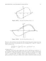
... have Numerical Methods for Ordinary Differential Equations, Second Edition J C Butcher © 2008 John Wiley & Sons, Ltd ISBN: 978-0-470-72335-7 52 NUMERICAL METHODS FOR ORDINARY DIFFERENTIAL EQUATIONS ... Lotka–Volterra equations (106a), (106b) in the form given in Exercise 12.1 38 NUMERICAL METHODS FOR ORDINARY DIFFERENTIAL EQUATIONS 13 Difference Equation Problems 130 Introduction to difference equations ... given by 32 NUMERICAL METHODS FOR ORDINARY DIFFERENTIAL EQUATIONS 102 Figure 121(ii) 1+ √ 2+ √ 2 √ √ 1+ √ 10 Solution to neutral delay differential equation (121c) the formula for y (x) for x positive...
Ngày tải lên: 13/08/2014, 05:21
Numerical Methods for Ordinary Dierential Equations Episode 3 pot
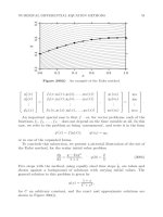
... which of various alternative numerical methods should be used for a specific problem, or even for a large class of problems 56 NUMERICAL METHODS FOR ORDINARY DIFFERENTIAL EQUATIONS Table 201(II) h ... 12 12 −9 NUMERICAL METHODS FOR ORDINARY DIFFERENTIAL EQUATIONS 0.05 h 0.10 0.15 62 Figure 203(iii) x Stepsize h against x for the ‘mildly stiff’ problem (203a) with variable stepsize for T = 0.02 ... function, y, on [x0 , x] by the formula y(x) = y(xk−1 ) + (x − xk−1 )f (xk−1 , y(xk−1 )), x ∈ (xk−1 , xk ], (210b) 66 NUMERICAL METHODS FOR ORDINARY DIFFERENTIAL EQUATIONS for k = 1, 2, , n If we...
Ngày tải lên: 13/08/2014, 05:21

Numerical Methods for Ordinary Dierential Equations Episode 4 doc
... converge for large stepsizes (not shown in the diagrams) This effect persisted for a larger range of stepsizes for PEC methods than was the case for PECE methods NUMERICAL METHODS FOR ORDINARY DIFFERENTIAL ... than for corresponding explicit NUMERICAL METHODS FOR ORDINARY DIFFERENTIAL EQUATIONS 10−6 10−4 104 −8 E 10 10 −10 10−4 Figure 239(ii) 10−3 h 10−2 Runge–Kutta methods with cost corrections methods ... with Figure 252(i) shows the new methods to be slightly more accurate for the same stepsizes 122 NUMERICAL METHODS FOR ORDINARY DIFFERENTIAL EQUATIONS The final numerical result in this subsection...
Ngày tải lên: 13/08/2014, 05:21

Numerical Methods for Ordinary Dierential Equations Episode 5 docx
... by Numerical Methods for Ordinary Differential Equations, Second Edition J C Butcher © 2008 John Wiley & Sons, Ltd ISBN: 978-0-470-72335-7 138 NUMERICAL METHODS FOR ORDINARY DIFFERENTIAL EQUATIONS ... 124 NUMERICAL METHODS FOR ORDINARY DIFFERENTIAL EQUATIONS 262 Generalized linear multistep methods These methods, known also as hybrid methods or modified linear multistep methods, generalize ... interpolation formula in the form y(xn−1 + ht) ≈ (1 + 2t)(1 − t)2 y(xn−1) + (3 − 2t)t2 y(xn ) + t(1 − t)2 hy (xn−1 ) − t2 (1 − t)hy (xn ) 132 NUMERICAL METHODS FOR ORDINARY DIFFERENTIAL EQUATIONS...
Ngày tải lên: 13/08/2014, 05:21

Numerical Methods for Ordinary Dierential Equations Episode 6 ppsx
... of the matrix A For i corresponding to a member of row k for k = 1, 2, , m, the only non-zero 190 NUMERICAL METHODS FOR ORDINARY DIFFERENTIAL EQUATIONS aij are for j = and for j corresponding ... ) For explicit methods, D(2) cannot hold, for similar reasons to the impossibility of C(2) For implicit methods D(s) is possible, as we shall see in Section 342 174 NUMERICAL METHODS FOR ORDINARY ... 31.3 For an arbitrary Runge–Kutta method, find the order condition corresponding to the tree 170 NUMERICAL METHODS FOR ORDINARY DIFFERENTIAL EQUATIONS 32 Low Order Explicit Methods 320 Methods...
Ngày tải lên: 13/08/2014, 05:21
Numerical Methods for Ordinary Dierential Equations Episode 7 potx
... p + (333g) 204 NUMERICAL METHODS FOR ORDINARY DIFFERENTIAL EQUATIONS Proof For a given tree t, let Φ(t) denote the elementary weight for (333a) and Φ(t) the elementary weight for (333b) Because ... I formula, c1 = This formula is exact for polynomials of degree up to 2s − II For the Radau II formula, cs = This formula is exact for polynomials of degree up to 2s − III For the Lobatto formula, ... of degree 216 NUMERICAL METHODS FOR ORDINARY DIFFERENTIAL EQUATIONS ∗ less than n − A simple calculation shows that Q is orthogonal to Pk for ∗ k < n − Hence, (342f) follows except for the value...
Ngày tải lên: 13/08/2014, 05:21

Numerical Methods for Ordinary Dierential Equations Episode 8 ppsx
... 230 NUMERICAL METHODS FOR ORDINARY DIFFERENTIAL EQUATIONS 35 Stability of Implicit Runge–Kutta Methods 350 A-stability, A(α)-stability and L-stability We recall that the stability function for ... choose Z = −t diag(ej ), for t positive The value of R(Z) becomes R(Z) = − tbj + O(t2 ), 248 NUMERICAL METHODS FOR ORDINARY DIFFERENTIAL EQUATIONS which is greater than for t sufficiently small Now ... non-linear equations We consider how to solve these equations using a full Newton method This requires going through the following steps: 260 NUMERICAL METHODS FOR ORDINARY DIFFERENTIAL EQUATIONS...
Ngày tải lên: 13/08/2014, 05:21

Numerical Methods for Ordinary Dierential Equations Episode 9 ppsx
... Runge–Kutta methods exist for which A is lower triangular? 280 NUMERICAL METHODS FOR ORDINARY DIFFERENTIAL EQUATIONS 38 Algebraic Properties of Runge–Kutta Methods 380 Motivation For any specific ... then the sub-forest induced by V is the forest (V , E), where E is the intersection of V × V and E A special 288 NUMERICAL METHODS FOR ORDINARY DIFFERENTIAL EQUATIONS case is when a sub-forest (V ... acceptable for many problems In each of the values of ξ for which there is a single underline, the method is A(α)-stable with α ≥ 1.55 ≈ 89◦ 268 NUMERICAL METHODS FOR ORDINARY DIFFERENTIAL EQUATIONS...
Ngày tải lên: 13/08/2014, 05:21

Numerical Methods for Ordinary Dierential Equations Episode 10 pot
... requirements Numerical Methods for Ordinary Differential Equations, Second Edition J C Butcher © 2008 John Wiley & Sons, Ltd ISBN: 978-0-470-72335-7 318 NUMERICAL METHODS FOR ORDINARY DIFFERENTIAL EQUATIONS ... therefore over several steps 322 NUMERICAL METHODS FOR ORDINARY DIFFERENTIAL EQUATIONS 405 Necessity of conditions for convergence We formally prove that stability and consistency are necessary for ... each of them and methods can be constructed which also lie in them We first prove the following result: 302 NUMERICAL METHODS FOR ORDINARY DIFFERENTIAL EQUATIONS Theorem 388H For any real θ and...
Ngày tải lên: 13/08/2014, 05:21

Numerical Methods for Ordinary Dierential Equations Episode 11 pptx
... of this test in Subsection 433 346 NUMERICAL METHODS FOR ORDINARY DIFFERENTIAL EQUATIONS Algorithm 432α Boundary locus method for low order Adams–Bashforth methods % Second order % -w = ... 348 NUMERICAL METHODS FOR ORDINARY DIFFERENTIAL EQUATIONS 2i −6 −4 −2 −2i Figure 432(iii) Stability region for the third order Adams–Moulton method 2i −2i Figure 432(iv) Stability region for ... following equations for the predicted and corrected values: ∗ ∗ ∗ yn = yn−1 + hfn−1 − hfn−2 , (434a) 2 ∗ ∗ (434b) yn = yn−1 + hfn + hfn−1 2 350 NUMERICAL METHODS FOR ORDINARY DIFFERENTIAL EQUATIONS...
Ngày tải lên: 13/08/2014, 05:21

Numerical Methods for Ordinary Dierential Equations Episode 12 pptx
... yr Numerical Methods for Ordinary Differential Equations, Second Edition J C Butcher © 2008 John Wiley & Sons, Ltd ISBN: 978-0-470-72335-7 374 NUMERICAL METHODS FOR ORDINARY DIFFERENTIAL EQUATIONS ... one of these formulations, can be transformed into the sequence that would have been generated using the alternative formulation 376 NUMERICAL METHODS FOR ORDINARY DIFFERENTIAL EQUATIONS It ... linear formulation from the start, and then explore the existence of suitable methods that have no connection with linear multistep methods 382 NUMERICAL METHODS FOR ORDINARY DIFFERENTIAL EQUATIONS...
Ngày tải lên: 13/08/2014, 05:21

Numerical Methods for Ordinary Dierential Equations Episode 13 pps
... form given by Exercise 53.1 420 NUMERICAL METHODS FOR ORDINARY DIFFERENTIAL EQUATIONS 54 Methods with Runge–Kutta stability 540 Design criteria for general linear methods We consider some of the ... NUMERICAL METHODS FOR ORDINARY DIFFERENTIAL EQUATIONS stability properties that are usually superior to those of alternative methods For example, A-stability is inconsistent with high order for ... V as a simple matrix, for example a matrix with rank 422 NUMERICAL METHODS FOR ORDINARY DIFFERENTIAL EQUATIONS If p = q, it is a simple matter to write down conditions for this order and stage...
Ngày tải lên: 13/08/2014, 05:21

Numerical Methods for Ordinary Dierential Equations Episode 14 pdf
... 18 Numerical Methods for Ordinary Differential Equations, Second Edition J C Butcher © 2008 John Wiley & Sons, Ltd ISBN: 978-0-470-72335-7 460 NUMERICAL METHODS FOR ORDINARY DIFFERENTIAL EQUATIONS ... Hybrid methods for initial value problems in ordinary differential equations SIAM J Numer Anal., 2, 69–86 456 NUMERICAL METHODS FOR ORDINARY DIFFERENTIAL EQUATIONS Gear C W (1967) The numerical ... (2002) and Butcher and Wright (2003, 2003a) 446 NUMERICAL METHODS FOR ORDINARY DIFFERENTIAL EQUATIONS 555 Some non-stiff methods The following method, for which c = [ , , 1] , has order 2: 3 ...
Ngày tải lên: 13/08/2014, 05:21

Computer Methods for Ordinary Differential Equations and Differential Algebraic Equations
... relevant for computer methods, Chapter introduces all the basic concepts and simple methods (relevant also for boundary value problems and for DAEs), Chapter is devoted to one-step (Runge-Kutta) methods ... solutions for Example 9.9 252 9.4 A matrix in Hessenberg form 258 10.1 Methods for the direct discretization of DAEs in general form 265 10.2 Maximum errors for ... path for (x2 y2) 290 ; Chapter Ordinary Di erential Equations Ordinary di erential equations (ODEs) arise in many instances when using mathematical modeling techniques for describing...
Ngày tải lên: 21/12/2016, 10:35

Tài liệu Numerical Methods for Ordinary Differential Equations pptx
... Numerical Methods for Ordinary Differential Equations Numerical Methods for Ordinary Differential Equations, Second Edition J C Butcher © 2008 John Wiley & Sons, Ltd ISBN: 978-0-470-72335-7 Numerical ... which Numerical Methods for Ordinary Differential Equations, Second Edition J C Butcher © 2008 John Wiley & Sons, Ltd ISBN: 978-0-470-72335-7 NUMERICAL METHODS FOR ORDINARY DIFFERENTIAL EQUATIONS ... in detail the design of efficient explicit methods for non-stiff xiv NUMERICAL METHODS FOR ORDINARY DIFFERENTIAL EQUATIONS problems For implicit methods for stiff problems, inexpensive implementation...
Ngày tải lên: 13/02/2014, 20:20

Numerical Methods for Ordinary Differential Equations pdf
... Numerical Methods for Ordinary Differential Equations Numerical Methods for Ordinary Differential Equations, Second Edition J C Butcher © 2008 John Wiley & Sons, Ltd ISBN: 978-0-470-72335-7 Numerical ... which Numerical Methods for Ordinary Differential Equations, Second Edition J C Butcher © 2008 John Wiley & Sons, Ltd ISBN: 978-0-470-72335-7 NUMERICAL METHODS FOR ORDINARY DIFFERENTIAL EQUATIONS ... in detail the design of efficient explicit methods for non-stiff xiv NUMERICAL METHODS FOR ORDINARY DIFFERENTIAL EQUATIONS problems For implicit methods for stiff problems, inexpensive implementation...
Ngày tải lên: 27/06/2014, 05:20

Numerical Methods for Ordinary Differential Equations Numerical Methods pptx
... Numerical Methods for Ordinary Differential Equations Numerical Methods for Ordinary Differential Equations, Second Edition J C Butcher © 2008 John Wiley & Sons, Ltd ISBN: 978-0-470-72335-7 Numerical ... which Numerical Methods for Ordinary Differential Equations, Second Edition J C Butcher © 2008 John Wiley & Sons, Ltd ISBN: 978-0-470-72335-7 NUMERICAL METHODS FOR ORDINARY DIFFERENTIAL EQUATIONS ... in detail the design of efficient explicit methods for non-stiff xiv NUMERICAL METHODS FOR ORDINARY DIFFERENTIAL EQUATIONS problems For implicit methods for stiff problems, inexpensive implementation...
Ngày tải lên: 27/06/2014, 18:20

hilbert space methods for partial differential equations - r. showalter
... Semigroups Parabolic Equations V Implicit Evolution Equations Introduction Regular Equations Pseudoparabolic Equations Degenerate Equations Examples ... so that j C0 j (x) for all x Rn , supp( j ) Gj , and j (x) = for x Fj LetS C0 (Rn ) be chosen with (x) n , supp( ) G for all x R fFj : j N g, and (x) P for x G = Finally, for each j , j N , ... Approximation of Evolution Equations Introduction Regular Equations Sobolev Equations Degenerate Equations Examples ...
Ngày tải lên: 31/03/2014, 15:56
Bạn có muốn tìm thêm với từ khóa:
- systems of ordinary differential equations examples
- power series solution of ordinary differential equations
- system of ordinary differential equations second order
- system of ordinary differential equations mathematica
- coupled ordinary differential equations examples
- nonlinear ordinary differential equations examples