weighted 2 mixed sensitivity design for unstable system with time delay
báo cáo hóa học:" Research Article The Permanence and Extinction of a Discrete Predator-Prey System with Time Delay and Feedback Controls" ppt
... α0 , 3 .27 for n > n2 Let v n be the solution of 3 .21 with initial condition v n2 comparison theorem, we have u1 n ≥ v n , In 3 .22 , we choose n0 n2 and v0 v n for all n ≥ n2 ∀n ≥ n2 u1 n2 , by ... have −d n a21 n x∗ n − τ − ε3 − a 22 n 2 − c2 n ε3 > 2 β n x∗ n − τ − ε3 γ n 2 3.61 Considering the following equation with parameter α1 : Δv n −e2 n v n f2 n α1 , 3. 62 by Lemma 2. 4, for given ... that a 12 n − M 2 γ n ≡ for all n > n , otherwise α1 < max{ 2 , δ3 / f2 , 2 / a 12 n − 2 γ n M } Obviously, there exists an n2 > n1 , such that a 12 n α1 < 2 , γ n α1 f2 n α1 < δ3 , ∀n > n2 3.64...
Ngày tải lên: 21/06/2014, 11:20
Báo cáo hoa học: " Research Article Permanence of a Discrete n-Species Schoener Competition System with Time Delays and Feedback Controls" pptx
... cooperative system is more appropriate, and they proposed the following system: x1 k x2 k x1 k exp r1 k − x1 k − c1 k x1 k b1 k x2 k , x2 k − c2 k x1 k x2 k exp r2 k − a2 k b2 k x2 k a1 k 1.3 ... γil for all k ≥ K2 max{σi , i 1, 2, , n} Noticing that < 1−αu < i i Lemmas 2. 2 and 2. 3, it follows from 2. 41 that lim inf μi k ≥ βil mi − ε γil αu i k→ ∞ 2. 41 1, 2, , n , by applying 2. 42 ... Mi ε 1, 2, , n , by applying 2. 21 : Qi 2. 22 αli k→ ∞ 2. 20 Setting ε → in the inequality above leads to lim sup μi k ≤ βiu k→ ∞ γiu Mi αli This completes the proof of Proposition 2. 5 Now...
Ngày tải lên: 21/06/2014, 20:20
Collaborative fixture design and analysis system with robustness for machining parts
... 19 2. 3.1 Optimization Methods 20 2. 3 .2 Fixture Design Model for Robustness 22 2. 4 Problem Statement and Research Objectives 25 2. 4.1 Problem Statement 28 ... Collaborative Design Systems 9 2. 1.1 Collaboration Scenarios 10 2. 1 .2 Distributed Systems Architectures 12 2. 2 Ontology Modelling 16 2. 3 Robust Fixture Design ... 1 12 Figure 7 .2 The direction at local contact point 114 Figure 7.3 The representation for fixture design 122 Figure 7.4 Encoding of fixture design with 3 -2- 1 approach 123 ...
Ngày tải lên: 11/09/2015, 09:57

design of feedback control systems for unstable plants with saturating actuators
Ngày tải lên: 13/07/2016, 10:27

Báo cáo hóa học: " Research Article Description of a 2-Bit Adaptive Sigma-Delta Modulation System with Minimized Idle Tones" docx
... SDM −100 20 0 20 0 −300 Power spectral density (dB) −100 Power spectral density (dB) SDM 2- bit ASDM −100 20 0 −300 Proposed 2- bit ASDM −300 2- bit ASDM −100 −150 20 0 25 0 Proposed 2- bit ASDM ... −150 20 0 20 0 −300 100 101 1 02 103 Frequency (Hz) 104 25 0 105 1000 20 00 3000 4000 5000 6000 7000 8000 9000 Frequency (Hz) (a) (b) ×105 SDM Power 2 2-bit ASDM −1 2 1.5 0.5 −0.5 Proposed 2- bit ... SDM −100 20 0 20 0 −300 Power spectral density (dB) −100 Power spectral density (dB) SDM 2- bit ASDM −100 20 0 −300 Proposed 2- bit ASDM −300 2- bit ASDM −100 −150 20 0 25 0 Proposed 2- bit ASDM...
Ngày tải lên: 22/06/2014, 19:20
Báo cáo " Stability Radii for Difference Equations with Time-varying Coefficients " ppt
... is √ −162t + 162t2 + 61 + 324 t2 − 324 t + 97 2( 81t4 − 162t3 + 117t2 − 36t + 4) Hence, √ 61 √ −162t + 162t2 + 61 + 324 t2 − 324 t + 97 −1 = + sup (tI − B) = sup 97 2( 81t4 − 162t3 + 117t2 − 36t + ... stable Further The matrix (tI − B)−1 = 9t 2 9t2−9t +2 − 9t2 −9t +2 − 9t2 −9t +2 9t−7 9t2 −9t +2 184 L.H Lan / VNU Journal of Science, Mathematics - Physics 26 (20 10) 175-184 We know that (tI − B)−1 is ... stability radius of the unstructured system Xn+1 = 2 Xn −1 ∀n (23 ) 2 has two eigenvalues λ1 = 1/3 and 2 = 2/ 3 which line in the unit ball −1 Therefore, the system (23 ) is asymptotically stable Further...
Ngày tải lên: 22/03/2014, 11:20

Báo cáo hóa học: " Research Article Linear Impulsive Periodic System with Time-Varying Generating Operators on Banach Space" pot
... Lemma 2. 2 and Assumption 2. 6, (t,θ) ∈ Lb (X), for ≤ θ ≤ t ≤ T0 By (6) of Lemma 2. 5 and Assumption 2. 6, (t + T0 ,θ + T0 ) = (t,θ), for ≤ θ ≤ t ≤ T0 By (2) of Lemma 2. 2, (6) of Lemma 2. 5 and ... L|t − θ |α for t,θ,τ ∈ 0,T0 (2. 4) Lemma 2. 2 (see [23 ], page 159) Under Assumption 2. 1, the Cauchy problem ˙ x(t) + A(t)x(t) = 0, t ∈ 0,T0 with x(0) = x0 (2. 5) has a unique evolution system {U(t,θ) ... impulsive periodic system with time- varying generating operators and introduce the suitable definition of T0 -periodic PC-mild solution for homogeneous linear impulsive periodic system with time- varying...
Ngày tải lên: 22/06/2014, 19:20

Báo cáo nghiên cứu khoa học: "Stability Radii for Difference Equations with Time-varying Coefficients" docx
... is √ −162t + 162t2 + 61 + 324 t2 − 324 t + 97 2( 81t4 − 162t3 + 117t2 − 36t + 4) Hence, √ 61 √ −162t + 162t2 + 61 + 324 t2 − 324 t + 97 −1 = + sup (tI − B) = sup 97 2( 81t4 − 162t3 + 117t2 − 36t + ... stable Further The matrix (tI − B)−1 = 9t 2 9t2−9t +2 − 9t2 −9t +2 − 9t2 −9t +2 9t−7 9t2 −9t +2 184 L.H Lan / VNU Journal of Science, Mathematics - Physics 26 (20 10) 175-184 We know that (tI − B)−1 is ... stability radius of the unstructured system Xn+1 = 2 Xn −1 ∀n (23 ) 2 has two eigenvalues λ1 = 1/3 and 2 = 2/ 3 which line in the unit ball −1 Therefore, the system (23 ) is asymptotically stable Further...
Ngày tải lên: 21/07/2014, 16:21

a novel scheme for human-friendly and time-delays robust neuropredictive teleoperation
... Athens, Greece, July 1998 HUMAN-FRIENDLY TIME- DELAYS ROBUST NEUROPREDICTIVE TELEOPERATION 12 13 14 15 16 17 18 19 20 21 22 23 24 25 26 27 28 29 30 31 32 33 339 Prokopiou, P A., Harwin, W S., and ... antagonist with height 30) for all plots (a) System G2 , free space (b) System G2 , contact with an object, modeled as a spring with Ke = 40 N/rad contacted at 72 deg (c) Free space With the enhanced ... (i) time- lead of the slave, which offers robustness to time delay without spoiling the reflected force- and reaction time for correcting errors or achieving compliance, and HUMAN-FRIENDLY TIME- DELAYS...
Ngày tải lên: 26/10/2014, 14:31

exponential attractors for a class of reaction difusion problems with time delay
... equations and delay models in population dynamics, Springer-Verlag Berlin Heidelberg, 1977 666 [13] [14] [15] [16] [17] [18] [19] [20 ] [21 ] [22 ] [23 ] [24 ] [25 ] [26 ] [27 ] [28 ] [29 ] [30] [31] [ 32] [33] ... i , P ψ˜ i ∈ Ej , for i = 1, This means P ψ˜ − P ψ˜ Z ≤ 2 ε, and (5 .2) entails ψ − 2 X = S( )ψ˜ − S( )ψ˜ ≤ e−γ ψ˜ − ψ˜ 2 X X + P ψ˜ − P ψ˜ 2 Z ≤ e−γ (2 )2 + (2 ε )2 = (2 θ )2 We can eventually ... ) 2 τ + d0 w s 1 ,2 ≤ w (s) 2 τ +c w s 2 τ + wt s X dt 2 Using (3.1) and (3 .2) , we deduce τ w s 2 τ + wt s X dt ≤ c w0 X τ + w 2 Hence w (τ ) 2 τ + d0 w 1 ,2 ≤ w (s) 2 +c w0 X τ + w Vol 7, 20 07...
Ngày tải lên: 29/10/2015, 14:19

attractors for differential equations with unbounded delays
... e(2d0 −λ1 )s γ 02 ds 1 /2 ψ 1 /2 e−(2d0 −λ1 )s γ 02 ds L2V ψ L2V γ0 ψ L2 =: K 1 /2 ψ V (2d0 − λ1 )1 /2 where we have used d0 > λ1 Therefore, F2 (t , ψ) 2 1 ≤ 2K ψ 2L2 , for ψ ∈ L2V , ≤ L2V , V so (8) ... F2 (t , 2 ) − F2 (t , ψ1 ) −1 ≤ −∞ ed0 r 2 (r ) − ψ1 (r ) = γ0 −∞ ∞ ≤ γ0 dr 1 /2 e−(2d0 −λ1 )r dr 2 − ψ1 γ0 2 − ψ1 (2d0 − λ1 )1 /2 = L2V L2V For condition (10), we note that ,for any ψ ∈ L2 ... ) dr ds −∞ τ 2 02 d0 s eλ1 s τ 2 02 d0 γ0 e−d0 (s−r ) u(r ) dr −∞ t ≤ 2 02 ≤ s eλ1 s −∞ τ t τ eλ1 s e−d0 (s−r ) u(r ) t ed0 r u(r ) −∞ τ 2 02 d0 (d0 − λ1 ) 2 02 d0 (d0 − λ1 ) 2 02 −∞ τ d0 (d0...
Ngày tải lên: 29/10/2015, 14:20

attractors for differential equations with unbounded delays
... Then d x(τ ) dτ 2 2 x(τ ) + 2 , and so d 2 τ x(τ ) e dτ 2e2ατ β Therefore, integrating over [s, τ ] with τ ∈ [s, t] τ e 2 τ x(τ ) e 2 s x(s) + 2 e2αρ dρ s = e2αs ϕ(0) + β 2 τ e − e2αs α Notice ... equations with delays, J Differential Equations 20 8 (1) (20 05) 9–41 [10] T Caraballo, J Real, Attractors for 2D-Navier–Stokes models with delays, J Differential Equations 20 5 (20 04) 27 1 29 7 [11] ... d2 + − e(2m1 −λ)(t−t0 ) k2 (e2γ h − eλh ) λh [e (1 − ρ∗ )]1 /2 (2 − λ) e(2m1 −λ)(t−t0 ) t e(2m1 −λ)(t−r) β(r) dr +2 t0 Now, we use the condition 2m1 − λ < and (21 ) or (22 ) to finish the proof ✷...
Ngày tải lên: 29/10/2015, 14:20

Using EPANET for irrigation system design
... 0.5 for sprinklers/nozzles Calculate the Emitter Coeficients for the Varying Nozzles For the rainbird 30H (SBN-3) with plug @ 50 psi: 9/64” nozzle, C = q/p0.5 = 4.1 gpm/ 500.5 = 0.580 5/ 32 nozzle, ... system Demand declines and the VFD lowers the pump speed to 320 0 rpm What are the power savings? P1 = 10 hp N1 = 3600 rpm N2 = 320 0 rpm P2 = hp An 11.1% speed decrease results in a 30% decrease in ... Selection Software, Q = 350 gpm, TDH = 21 5 ft Power, hydraulic (water) : 18.97 hp Power, brake : 26 .90 hp Minimum recommended driver rating set @ : 30.00 hp / 22 .37 kW Electronic Variable Frequency...
Ngày tải lên: 08/03/2014, 17:44
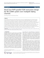
Báo cáo hóa học: "Novel low-PAPR parallel FSOK transceiver design for MC-CDMA system over multipath fading channels" pdf
... SC-FDMA systems under the same data rate scenario For example, the proposed QPSK-FSOK system (N = 4, P = 8, K = 4) with (log2N + 2) PK = 128 bits/sym, the conventional MC-CDMA system (M = 128 , P ... with 2KP = 128 bits/sym, and the interleaved SC-FDMA system (Q = 2, P = 16, K = 4) with 2KP = 128 bits/sym all have the same user data rates and total number of subcarriers M = NPK = QPK = 128 ... algorithms for LTE SC-FDMA based uplink MIMO systems IEEE Trans Wirel Commun 9(1), 60–65 (20 10) 21 H Harada, R Prasad, Simulation and Software Radio for Mobile Communications (Artech-House, 20 02) 22 JG...
Ngày tải lên: 20/06/2014, 22:20

Báo cáo hóa học: " Research Article A New Hybrid Algorithm for a System of Mixed Equilibrium Problems, Fixed Point Problems for Nonexpansive Semigroup, and Variational Inclusion Problem" ppt
... C4 {αn } ⊂ c, d , for some c, d ∈ ξ, ; C5 {λn } ⊂ a1 , b1 , for some a1 , b1 ∈ 0, 2 ; C6 {δn } ⊂ a2 , b2 , for some a2 , b2 ∈ 0, 2 ; C7 lim infn → ∞ rk,n > 0, for each k ∈ 1, 2, 3, , N Then, ... some c, d ∈ ξ, ; C5 {λn } ⊂ a1 , b1 , for some a1 , b1 ∈ 0, 2 ; C6 {δn } ⊂ a2 , b2 , for some a2 , b2 ∈ 0, 2 ; C7 lim infn → ∞ rk,n > 0, for each k ∈ 1, 2, 3, , N Then, {xn } and {un } converge ... some c, d ∈ ξ, ; C5 {λn } ⊂ a1 , b1 , for some a1 , b1 ∈ 0, 2 ; C6 {δn } ⊂ a2 , b2 , for some a2 , b2 ∈ 0, 2 ; C7 lim infn → ∞ rk,n > 0, for each k ∈ 1, 2, 3, , N Then, {xn } and {un } converge...
Ngày tải lên: 21/06/2014, 07:20

Báo cáo hóa học: " Research Article Algorithms of Common Solutions to Generalized Mixed Equilibrium Problems and a System of Quasivariational Inclusions for Two Difference Nonlinear Operators in Banach Spaces" pdf
... JM2 , 2 x∗ − 2 A2 x∗ , x∗ , y∗ is a solution of the problem 1.1 if and only if x∗ is a fixed point of the mapping Q defined by Q x J M1 ,ρ1 J M2 , 2 x − 2 A2 x − ρ1 A1 J M2 , 2 x − 2 A2 x 1 .28 ... fact that J M2 , 2 and I − 2 A2 are nonexpansive mappings, we get yn − y J M2 , 2 un − 2 A2 un − J M2 , 2 x − 2 A2 x ≤ u n − ρ A un − x − ρ A x I − ρ A2 u n − I − ρ A2 x 3.6 ≤ un − x ≤ xn − x ... ρ1 A1 yn − p − ρ1 A1 p ≤ yn − p J M2 , 2 un − 2 A2 un − J M2 , 2 p − 2 A2 p ≤ u n − ρ A un − p − ρ A p ≤ un − p 3 .26 From 3 .25 and 3 .26 , we have en − p 2 ≤ μ1 Sk xn − p − μ1 ≤ μ1 xn − p −...
Ngày tải lên: 21/06/2014, 07:20
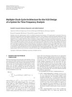
Báo cáo hóa học: " Multiple-Clock-Cycle Architecture for the VLSI Design of a System for Time-Frequency Analysis" doc
... us SM/Load STFT RESET Interval: 2. 32 us us Value: CumADD and OutREG CEIL(log2 ( (22 l+1 − 1) · (Ld max + 1))) 0 SelSTFT[8 0] D 18 18 26 7 26 0 64 18 26 7 26 0 64 18 26 7 26 0 64 ShLorNo[0] D0 1 0 1 0 1 ... 0] 18 26 7 26 0 64 18 26 7 26 0 64 18 26 7 26 0 1 0 1 0 1 36 49 145 23 5 64 D0 106 25 106 190 23 5 (b) Figure 11: Simulation illustration for test vector V = {5, 6, 7, 8, 9, 0, 0, } and Ld = 4 .2 Implementation ... EPF10K100GC5033DX49 92 66% EP20K200 Real + Imag 8-bits MCI 128 1 198 144 69 74% EPF10K30RC208-3 Real + Imag 8-bits SCI 35 32 150 57 94% EPF10K70RC240 -2 Real + Imag 16-bits MCI 3543 397 144 125 94% EPF10K70RC248-3...
Ngày tải lên: 22/06/2014, 23:20
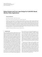
Báo cáo hóa học: "Robust System and Cross-Layer Design for H.264/AVC-Based Wireless Video Applications" pptx
... PSNR (dB) 36 Foreman QCIF, 7.5 fps over UMTS dedicated channel with LLC loss rate 10% 30 28 26 30 28 26 24 24 22 22 20 60 20 100 150 20 0 500 1000 20 00 (1) UM, Smax = 50, p = 0% (2) UM, RDO p ... 34 Average PSNR (dB) Foreman QCIF, 7.5 fps over UMTS dedicated channel with LLC loss rate 10% 30 28 26 24 30 28 26 24 22 22 20 60 100 150 20 0 500 1000 20 00 Initial playout delay Δ (ms) (1) UM, ... 34 35 33 32 33 PSNR (dB) PSNR (dB) 34 32 31 31 30 30 29 29 28 28 10 20 30 40 AL throughput ηAL (kbp/s) 50 27 60 26 Fragmentation 600, TTI = 80 ms Single slice mode, TTI = 80 ms FMO 2, TTI = 80...
Ngày tải lên: 22/06/2014, 23:20

Báo cáo hóa học: " Multilevel LDPC Codes Design for Multimedia Communication CDMA System" docx
... 26 , 21 } { 12, 24 , 17, 3, 6} {13, 26 , 21 , 11, 22 } {14, 28 , 25 , 19, 7} {15, 30, 29 , 27 , 23 } B1,1 B1 ,2 B1,3 B1,4 16 B1,5 B2,1 B2 ,2 12 B2,3 24 B2,4 17 B2,5 B3,1 10 B3 ,2 20 B3,3 B3,4 18 B3,5 Figure 6: ... and the information vector of the codeword vector, u, such that p p d d H u =H u {6, 12, 24 , 17, 3} {7, 14, 28 , 25 , 19} {9, 18, 5, 10, 20 } {10, 20 , 9, 18, 5} {11, 22 , 13, 26 , 21 } { 12, 24 , 17, ... 0(mod 31) · 2ms = 1(mod 31) · 2ms = 3(mod 31) · 2ms = 5(mod 31) · 2ms = 6(mod 31) · 2ms = 7(mod 31) · 2ms = 9(mod 31) 10 · 2ms = 10(mod 31) 11 · 2ms = 11(mod 31) 12 · 2ms = 12( mod 31) 13 · 2ms = 13(mod...
Ngày tải lên: 23/06/2014, 00:20
