solution methods for partial differential equations

hilbert space methods for partial differential equations - r. showalter
... well-posed These include boundary value problems for (stationary) elliptic partial di erential equations and initial-boundary value problems for (time-dependent) equations of parabolic, hyperbolic, and ... Semigroups Parabolic Equations V Implicit Evolution Equations Introduction Regular Equations Pseudoparabolic Equations Degenerate Equations Examples ... so that j C0 j (x) for all x Rn , supp( j ) Gj , and j (x) = for x Fj LetS C0 (Rn ) be chosen with (x) n , supp( ) G for all x R fFj : j N g, and (x) P for x G = Finally, for each j , j N ,...
Ngày tải lên: 31/03/2014, 15:56

Numerical Methods for Ordinary Differential Equations Butcher Tableau doc
... in detail the design of efficient explicit methods for non-stiff xiv NUMERICAL METHODS FOR ORDINARY DIFFERENTIAL EQUATIONS problems For implicit methods for stiff problems, inexpensive implementation ... Numerical Methods for Ordinary Differential Equations Numerical Methods for Ordinary Differential Equations, Second Edition J C Butcher © 2008 John Wiley & Sons, Ltd ISBN: 978-0-470-72335-7 Numerical Methods ... Numerical Methods for Ordinary Differential Equations, Second Edition J C Butcher © 2008 John Wiley & Sons, Ltd ISBN: 978-0-470-72335-7 NUMERICAL METHODS FOR ORDINARY DIFFERENTIAL EQUATIONS defines...
Ngày tải lên: 27/06/2014, 08:20

Partial Differential Equations part 1
... Ames, W.F 1977, Numerical Methods for Partial Differential Equations, 2nd ed (New York: Academic Press) [1] Richtmyer, R.D., and Morton, K.W 1967, Difference Methods for Initial Value Problems, ... different approaches to the solution of equation (19.0.10), not all applicable in all cases: relaxation methods, “rapid” methods (e.g., Fourier methods) , and direct matrix methods Sample page from ... conjugate gradient algorithm for solving finite-difference equations However, it is useful when incorporated in methods that first rewrite the equations so that A is transformed to a matrix A that...
Ngày tải lên: 28/10/2013, 22:15

Partial Differential Equations part 2
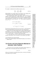
... Ames, W.F 1977, Numerical Methods for Partial Differential Equations, 2nd ed (New York: Academic Press), Chapter Richtmyer, R.D., and Morton, K.W 1967, Difference Methods for Initial Value Problems, ... Supplement, vol 55, pp 211–246, §2c [3] Kreiss, H.-O 1978, Numerical Methods for Solving Time-Dependent Problems for Partial Differential Equations (Montreal: University of Montreal Press), pp 66ff [4] ... or j 838 Chapter 19 Partial Differential Equations stable unstable ∆t ∆t ∆x ∆x x or j (a) ( b) Figure 19.1.3 Courant condition for stability of a differencing scheme The solution of a hyperbolic...
Ngày tải lên: 07/11/2013, 19:15

Tài liệu Partial Differential Equations part 3 pptx
... 19 Partial Differential Equations t or n (a) x or j Fully Implicit (b) (c) Crank-Nicholson Figure 19.2.1 Three differencing schemes for diffusive problems (shown as in Figure 19.1.2) (a) Forward ... diffusion problem, for example where D = D(u) Explicit schemes can be generalized in the obvious way For example, in equation (19.2.19) write 852 Chapter 19 Partial Differential Equations conditions ... method once again! CITED REFERENCES AND FURTHER READING: Ames, W.F 1977, Numerical Methods for Partial Differential Equations, 2nd ed (New York: Academic Press), Chapter Goldberg, A., Schey, H.M.,...
Ngày tải lên: 15/12/2013, 04:15
Tài liệu Partial Differential Equations part 4 ppt
... problems These will occupy us for the remainder of the chapter CITED REFERENCES AND FURTHER READING: Ames, W.F 1977, Numerical Methods for Partial Differential Equations, 2nd ed (New York: Academic ... 854 Chapter 19 Partial Differential Equations Lax Method for a Flux-Conservative Equation As an example, we show how to generalize the Lax method (19.1.15) to two dimensions for the conservation ... Reduction Methods for Boundary Value Problems As discussed in §19.0, most boundary value problems (elliptic equations, for example) reduce to solving large sparse linear systems of the form A·u=b...
Ngày tải lên: 15/12/2013, 04:15
Tài liệu Partial Differential Equations part 5 ppt
... 858 Chapter 19 Partial Differential Equations Fourier Transform Method The discrete inverse Fourier transform in both x and y is J−1 L−1 ujl = umn e−2πijm/J ... North America) ∂u = g(y) ∂x 862 Chapter 19 Partial Differential Equations The finite-difference form of equation (19.4.28) can be written as a set of vector equations uj−1 + T · uj + uj+1 = gj ∆2 ... and Cyclic Reduction Methods 859 • Compute ujl by the inverse Fourier transform (19.4.2) The above procedure is valid for periodic boundary conditions In other words, the solution satisfies ujl...
Ngày tải lên: 15/12/2013, 04:15
Tài liệu Partial Differential Equations part 6 doc
... radius of the Jacobi method For our model problem, therefore, 19.5 Relaxation Methods for Boundary Value Problems 867 • For this optimal choice, the spectral radius for SOR is ρSOR = ρJacobi + ... give a routine for SOR with Chebyshev acceleration 870 Chapter 19 Partial Differential Equations ADI (Alternating-Direction Implicit) Method The ADI method of §19.3 for diffusion equations can ... results, consider our model problem for which ρJacobi is given by equation (19.5.11) Then equations (19.5.19) and (19.5.20) give 868 Chapter 19 Partial Differential Equations Consider a general second-order...
Ngày tải lên: 15/12/2013, 04:15
Tài liệu Partial Differential Equations part 7 doc
... For example, Lh is the diagonal part of Lh for Jacobi iteration, or the lower triangle for Gauss-Seidel iteration The next approximation is generated by 874 Chapter 19 Partial Differential Equations ... Jespersen, D 1984, Multrigrid Methods for Partial Differential Equations (Washington: Mathematical Association of America) McCormick, S.F (ed.) 1988, Multigrid Methods: Theory, Applications, ... approximate solution is uH Then the coarse-grid correction is 884 Chapter 19 Partial Differential Equations • Fine grids are used to compute correction terms to the coarse-grid equations, yielding...
Ngày tải lên: 24/12/2013, 12:16

Functional analysis sobolev spaces and partial differential equations
... theorem, see Problem (b) In the theory of partial differential equations Let us mention, for example, that the existence of a fundamental solution for a general differential operator P (D) with constant ... Universitext For other titles in this series, go to www.springer.com/series/223 Haim Brezis Functional Analysis, Sobolev Spaces and Partial Differential Equations 1C Haim Brezis Distinguished ... Functional Analysis, Sobolev Spaces and Partial Differential Equations, DOI 10.1007/978-0-387-70914-7_2, © Springer Science+Business Media, LLC 2011 31 32 The Uniform Boundedness Principle and the...
Ngày tải lên: 04/02/2014, 11:10

Tài liệu AN INTRODUCTION TO PARTIAL DIFFERENTIAL EQUATIONS ppt
... This page intentionally left blank AN INTRODUCTION TO PARTIAL DIFFERENTIAL EQUATIONS A complete introduction to partial differential equations, this textbook provides a rigorous yet accessible ... selected exercises are included for students whilst extended solution sets are available to lecturers from solutions@cambridge.org AN INTRODUCTION TO PARTIAL DIFFERENTIAL EQUATIONS YEHUDA PINCHOVER ... of partial differential equations (PDEs) The book is suitable for all types of basic courses on PDEs, including courses for undergraduate engineering, sciences and mathematics students, and for...
Ngày tải lên: 16/02/2014, 15:20
Tài liệu Boundary Value Problems, Sixth Edition: and Partial Differential Equations pptx
... which they appear, and their solutions Our principal solution technique will involve separating a partial differential equation into ordinary differential equations Therefore, we begin by reviewing ... of assuming an exponential form for the solution works for linear homogeneous equations of any order with constant coefficients In all Chapter Ordinary Differential Equations Roots of Characteristic ... the entire solution of the given differential equation, not just to uc (t) Now we turn our attention to methods for finding particular solutions of nonhomogeneous linear differential equations...
Ngày tải lên: 17/02/2014, 14:20

Partial Differential Equations and Fluid Mechanics doc
... Cambridge University Press at www.cambridge.org/mathematics Stochastic partial differential equations, A ETHERIDGE (ed) Quadratic forms with applications to algebraic geometry and topology, A PFISTER ... Fern´ndez-Cara a 64 Singularity formation and separation phenomena in boundary layer theory F Gargano, M.C Lombardo, M Sammartino, & V Sciacca 81 Partial regularity results for solutions of the Navier–Stokes ... Navier–Stokes equations in a bounded cylindrical domain M Paicu & G Raugel 146 The regularity problem for the three-dimensional Navier–Stokes equations J.C Robinson & W Sadowski 185 Contour dynamics for...
Ngày tải lên: 14/03/2014, 10:20

Entropy and partial differential equations evans l c
... Euler equations in one dimension a Computing entropy/entropy flux pairs b Kinetic formulation VI Hamilton–Jacobi and related equations A Viscosity solutions B Hopf–Lax formula C A diffusion limit Formulation ... Conservation law form Boltzmann’s equation a A model for dilute gases b H-Theorem c H and entropy B Single conservation law Integral solutions Entropy solutions Condition E Kinetic formulation A ... other words we are assuming that formula (17), which we showed above holds for any Carnot heat engine for an ideal gas, in fact holds for any Carnot heat engine for our general homogeneous fluid...
Ngày tải lên: 17/03/2014, 14:29
harmonic analysis and partial differential equations - b. dahlberg, c. kenig
... of Theorem 1.4 47 Dirichlet Problem for Lipschitz domains The nal arguments for the L2-theory 51 Existence of solutions to Dirichlet and Neumann problems for Lipschitz domains The optimal Lp-results ... < such that j'(x) ? '(z)j M jx ? zj for all x and z y = '(x) x To solve the BVP:s we will reformulate the problems in terms of integral equations It therefore becomes necessary to study singular ... jP ? Q Q This estimate is uniform in P and Q since @ compact For f C (@ ) de ne Tf (P ) = Z @ K (P; Q)f (Q)d (Q); P @ : We can now formulate Lemma (jump relation for D) 1) D+ = I + T 2) D? =...
Ngày tải lên: 31/03/2014, 15:16
introduction to partial differential equations - a computational approach - a. tveito, r. winther
... of partial differential equations Therefore, a modern introduction to this topic must focus on methods suitable for computers But these methods often rely on deep analytical insight into the equations ... have chosen to study partial differential equations That decision is a wise one; the laws of nature are written in the language of partial differential equations Therefore, these equations arise as ... shall derive exact solutions for some partial differential equations Our purpose is to introduce some basic techniques and show examples of solutions represented by explicit formulas Most of the...
Ngày tải lên: 31/03/2014, 15:56


partial differential equations and the finite element method - pave1 solin
... transformations 7.2.3 Potential formulation of Maxwell’s equations 7.2.4 Other wave equations 7.2.5 7.3 Equations for the field vectors Equation for the electric field 7.3.1 7.3.2 Equation for ... others Equations involving partial derivatives are called partial diferential equations (PDEs) The solutions to these equations are functions, as opposed to standard algebraic equations whose solutions ... classical formulation (1.26), (1.28) In the language of linear forms Let V = HA(R) We define a bilinear form a(., ) VxV+Iw and a linear form E V ' , : 16 PARTIAL DIFFERENTIAL EQUATIONS Then the weak formulation...
Ngày tải lên: 31/03/2014, 15:57

partial differential equations, (ma3132 lecture notes) - b. neta (
... canonical form for hyperbolic α = ξ + η, β = ξ − η H∗ A∗ H∗ = ∗ C second canonical form for hyperbolic uξξ = uηη uαα + uββ = H ∗∗ A∗∗ a canonical form for parabolic a canonical form for parabolic ... derivatives Before we discuss transformation to canonical forms, we will motivate the name and explain why such transformation is useful The name canonical form is used because this form 15 corresponds ... another canonical form for hyperbolic PDEs which is obtained by making a transformation α =ξ+η (2.3.1.15) uξη = β = ξ − η (2.3.1.16) Using (2.3.1.6)-(2.3.1.8) for this transformation one has...
Ngày tải lên: 31/03/2014, 15:57

stochastic partial differential equations and applications - math da prato g , tubaro l
Ngày tải lên: 08/04/2014, 12:26