show leave behind display an invitation to adventure option 5

An Introduction to Financial Option Valuation: Mathematics, Stochastics and Computation_13 pot
... = 50 and Nt = 50 0, so k = × 10−3 and h = 0.2, we found that err0 = 1 .5 × 10−3 for FTCS and err0 = 1.7 × 10⁻³ for BTCS With Crank– Nicolson we were able to reduce Nt to 50 , so k = × 10−2 , and ... = 0.63 1 .5 0 .5 −0 .5 −1 −1 .5 100 80 15 60 10 40 20 t x Fig 23 .5 FTCS solution on the heat equation (23.2), (23.3) and (23.4) with initial and boundary conditions (23 .5) Here N x = 14 and Nt = ... > 23.7 Show that Crank–Nicolson, (23.18), can be expressed as 2 − νδx U i+1 = + νδx U ij j 2 23.8 By analogy with (23.13) and (23. 15) , define the local accuracy for Crank–Nicolson and show that...
Ngày tải lên: 20/06/2014, 18:20

An Introduction to Financial Option Valuation: Mathematics, Stochastics and Computation_14 pot
... 174, 1 75 ARCH, see autoregressive conditional heteroscedasticity Asian option, 192–194, 196 ask price, asset model continuous, 56 , 59 , 60 discrete, 54 , 55 , 60, 151 incremental, 56 mean, 56 , 60, ... 1 75, 182 liquidity, 94 log ratio, 48, 203, 210 lognormal distribution, 56 , 57 , 59 , 60, 66, 70, 118 London International Financial Futures and Options Exchange, 5, 1 35 London Stock Exchange, 50 ... option, 191 down-and-in call, 188, 189 down-and-in put, 190 down-and-out call, 187–189, 260–261, 2 65 down-and-out put, 190 drift, 54 , 1 05, 198 efficient market hypothesis, 45 46, 49, 51 , 52 , 54 ,...
Ngày tải lên: 20/06/2014, 18:20

An Introduction to Financial Option Valuation: Mathematics, Stochastics and Computation_1 pot
... method in practice 16 .5 Notes and references 16.6 Program of Chapter 16 and walkthrough 151 151 151 153 154 156 159 17 Cash-or-nothing options 17.1 Motivation 17.2 Cash-or-nothing options 17.3 Black–Scholes ... asset model 6.6 Notes and references 6.7 Program of Chapter and walkthrough 53 53 53 55 56 57 59 60 Asset price model: Part II 7.1 Computing asset paths 7.2 Timescale invariance 7.3 Sum-of-square ... paths and final time histogram xiii page 15 18 19 25 26 27 30 31 36 37 38 39 39 40 42 46 47 47 51 57 61 64 65 65 66 xiv 7 .5 7.6 7.7 8.1 8.2 9.1 9.2 9.3 9.4 9 .5 10.1 11.1 11.2 11.3 11.4 11 .5 11.6...
Ngày tải lên: 20/06/2014, 18:20
An Introduction to Financial Option Valuation: Mathematics, Stochastics and Computation_3 pptx
... to N(0, 1) ♦ 39 4.3 Statistical tests N(0,1) samples and N(0,1) quantiles N(0,1) samples and U(0,1) quantiles 5 0 5 5 5 5 U(0,1) samples and N(0,1) quantiles U(0,1) samples and U(0,1) quantiles ... (4.1) and sample variance (4.2) using M samples from a U(0, 1) and an N(0, 1) pseudo-random number generator U(0, 1) N(0, 1) M µM σM µM σM 102 103 104 1 05 0 .52 29 0.4884 0 .50 09 0 .50 10 0.0924 0.08 45 ... sample means and variances approach the true values and 12 ≈ 0.0833 (recall Exercise 3 .5) and the N(0, 1) sample means and variances approach the true values and A more enlightening approach to testing...
Ngày tải lên: 20/06/2014, 18:20

An Introduction to Financial Option Valuation: Mathematics, Stochastics and Computation_4 ppt
... (6.13) 6 .5 Features of the asset model 57 t =1 1 .5 σ = 0.3 σ = 0 .5 f (x) 0 .5 0 0 .5 1 .5 2 .5 3 .5 t =3 1 .5 σ = 0.3 σ = 0 .5 f (x) 0 .5 0 0 .5 1 .5 2 .5 3 .5 Fig 6.1 Lognormal density (6.10) for µ = 0. 05, S0 ... Density IBM Daily 0.4 0.3 0 .5 0.2 −2 0.1 5 5 IBM Weekly Rand Num Gen 5 0.3 0 .5 0.2 −2 0.1 5 −4 5 0.4 0.3 0 .5 0.2 −2 0.1 5 −4 − 5 0.4 5 Quantiles 5 −4 5 Fig 5. 3 Statistical tests of IBM ... www.maths.warwick.ac.uk/wiberg/MathFinance/ to manipulate and display real stock market data 5. 6 Program of Chapter and walkthrough 51 %CH 05 Program for Chapter % % Illustrates quantile plot clf randn(’state’,100)...
Ngày tải lên: 20/06/2014, 18:20
An Introduction to Financial Option Valuation: Mathematics, Stochastics and Computation_5 ppt
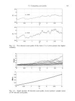
... Part II 2 .5 1 .5 0 .5 0 0.2 0.3 0.4 0 .5 0.6 0.7 0.8 0.9 0 .5 1 .5 2 .5 3 .5 4 .5 0.8 0.6 0.4 0.2 Fig 7.4 Upper picture: 50 discrete asset paths over [0, T ] with S0 = 1, µ = 0. 05, σ = 0 .5, T = and δt = ... S0 = 5, E = 4, T = 1, σ = 0.3 82 Black–Scholes PDE and formulas and r = 0. 05, we find, to four decimal places, d1 = 1.06 05, d2 = 0.76 05, N (d1 ) = 0. 855 5, N (d2 ) = 0.77 65, N (−d1 ) = 0.14 45, N ... the company and has many insights into the practical issues involved in collecting and analysing vast amounts of financial data EXERCISES 7.1 7.2 Confirm the results (7.4) and (7 .5) By analogy...
Ngày tải lên: 20/06/2014, 18:20
An Introduction to Financial Option Valuation: Mathematics, Stochastics and Computation_7 pdf
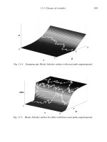
... , S for a call option, p := P , S for a put option and In these new variables, d1 and d2 in (8.20) and (8.21) simplify to d1 = m τ + τ and d2 = m τ − , τ (11.1) and, from (8.19) and (8.24), the ... applies to a European put option, as in Figure 11.4 P11.2 Edit ch11.m so that it applies to the delta of a European call option, as in Figure 11 .5, and investigate the use of surf, surfc and waterfall ... are close to an x and then switches to Newton’s method to get the benefit of rapid convergence Also, the residual |F(xn )| gives a measure of how close xn is to a solution, and this can be incorporated...
Ngày tải lên: 20/06/2014, 18:20

An Introduction to Financial Option Valuation: Mathematics, Stochastics and Computation_8 pptx
... was December 2001 136 Implied volatility Exercise price Option price 51 25 52 25 53 25 54 25 552 5 56 25 57 25 58 25 4 75 4 05 340 280 226 179 139 1 05 FTSE 100, 22 August, 2001 0.192 0.19 0.188 Implied volatility ... 0.172 51 00 52 00 53 00 54 00 55 00 56 00 57 00 58 00 59 00 Exercise price Fig 14.2 Implied volatility against exercise price for some FTSE 100 index data The initial asset price (on 22 August 2001) was 54 20.3 ... output provides an approximate option price a M and an approximate 95% confidence interval ( 15. 5) Computational example We now use the Monte Carlo method to value a European call option, so (S(T...
Ngày tải lên: 20/06/2014, 18:20

An Introduction to Financial Option Valuation: Mathematics, Stochastics and Computation_9 pot
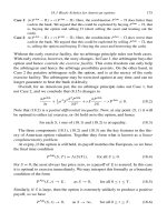
... put options 18.3 Black–Scholes for American options Our aim in this section is to show how the arguments in Chapter that led to the Black–Scholes PDE can be adapted to cover an American put option ... reach, and puts a strain on computational methods 18.2 American call and put An American option is like a European option except that the holder may exercise at any time between the start date and ... • American call and put equivalence of European and American call Black–Scholes for American put binomial method for American options optimal exercise boundary Monte Carlo for American options...
Ngày tải lên: 20/06/2014, 18:20

An Introduction to Financial Option Valuation_1 potx
... to N(0, 1) ♦ 39 4.3 Statistical tests N(0,1) samples and N(0,1) quantiles N(0,1) samples and U(0,1) quantiles 5 0 5 5 5 5 U(0,1) samples and N(0,1) quantiles U(0,1) samples and U(0,1) quantiles ... (4.1) and sample variance (4.2) using M samples from a U(0, 1) and an N(0, 1) pseudo-random number generator U(0, 1) N(0, 1) M µM σM µM σM 102 103 104 1 05 0 .52 29 0.4884 0 .50 09 0 .50 10 0.0924 0.08 45 ... sample means and variances approach the true values and 12 ≈ 0.0833 (recall Exercise 3 .5) and the N(0, 1) sample means and variances approach the true values and A more enlightening approach to testing...
Ngày tải lên: 21/06/2014, 04:20

An Introduction to Financial Option Valuation_2 potx
... (6.13) 6 .5 Features of the asset model 57 t =1 1 .5 σ = 0.3 σ = 0 .5 f (x) 0 .5 0 0 .5 1 .5 2 .5 3 .5 t =3 1 .5 σ = 0.3 σ = 0 .5 f (x) 0 .5 0 0 .5 1 .5 2 .5 3 .5 Fig 6.1 Lognormal density (6.10) for µ = 0. 05, S0 ... Density IBM Daily 0.4 0.3 0 .5 0.2 −2 0.1 5 5 IBM Weekly Rand Num Gen 5 0.3 0 .5 0.2 −2 0.1 5 −4 5 0.4 0.3 0 .5 0.2 −2 0.1 5 −4 − 5 0.4 5 Quantiles 5 −4 5 Fig 5. 3 Statistical tests of IBM ... www.maths.warwick.ac.uk/wiberg/MathFinance/ to manipulate and display real stock market data 5. 6 Program of Chapter and walkthrough 51 %CH 05 Program for Chapter % % Illustrates quantile plot clf randn(’state’,100)...
Ngày tải lên: 21/06/2014, 04:20
An Introduction to Financial Option Valuation_4 pot
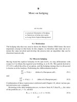
... More on hedging E 0 0 .5 1 .5 2 .5 3 .5 4 .5 0 .5 1 .5 2 .5 3 .5 4 .5 0 .5 1 .5 2 .5 3 .5 4 .5 0 .5 1 .5 2 .5 3 .5 4 .5 Delta 0 .5 Cash 1 .5 0 .5 Portfolio 2 .5 1 .5 Fig 9.1 Discrete hedging simulation Option expires in-the-money ... Delta at expiry E 0 0 .5 1 .5 2 .5 3 .5 4 .5 0 .5 1 .5 2 .5 3 .5 4 .5 0 .5 1 .5 2 .5 3 .5 4 .5 0 .5 1 .5 2 .5 3 .5 4 .5 Delta 0 .5 Cash 1 .5 0 .5 Portfolio 1 .5 Fig 9.2 Discrete hedging simulation Option expires out-of-the-money ... 9.4, and a similar financial argument applies, see Exercise 9 .5 (9.8) 92 Asset path More on hedging E 0 0 .5 1 .5 2 .5 3 .5 4 .5 0 .5 1 .5 2 .5 3 .5 4 .5 0 .5 1 .5 2 .5 3 .5 4 .5 0 .5 1 .5 2 .5 3 .5 4 .5 Delta 0 .5 Cash...
Ngày tải lên: 21/06/2014, 04:20

An Introduction to Financial Option Valuation_6 ppt
... was December 2001 136 Implied volatility Exercise price Option price 51 25 52 25 53 25 54 25 552 5 56 25 57 25 58 25 4 75 4 05 340 280 226 179 139 1 05 FTSE 100, 22 August, 2001 0.192 0.19 0.188 Implied volatility ... 0.172 51 00 52 00 53 00 54 00 55 00 56 00 57 00 58 00 59 00 Exercise price Fig 14.2 Implied volatility against exercise price for some FTSE 100 index data The initial asset price (on 22 August 2001) was 54 20.3 ... output provides an approximate option price a M and an approximate 95% confidence interval ( 15. 5) Computational example We now use the Monte Carlo method to value a European call option, so (S(T...
Ngày tải lên: 21/06/2014, 04:20
An Introduction to Financial Option Valuation_8 pdf
... 1.7983 1.7962 1.7962 177 18 .5 Optimal exercise boundary American put 1.82 1.8 15 1.81 1.8 05 1.8 1.7 95 50 100 150 200 250 M American put 1.79 85 1.798 1.79 75 1.797 1.79 65 1.796 200 220 240 260 280 ... Exercise 19.6 19 .5 Bermudan and shout options A Bermudan option differs from the corresponding American option in only one respect While the American option allows the holder to exercise at any time ... gives an approximate option price a M and an approximate 95% confidence interval ( 15. 5) For Asian options we could use the Riemann sum t N S j to approximate j=1 T the integral S(τ )dτ With an average...
Ngày tải lên: 21/06/2014, 04:20
An Introduction to Financial Option Valuation_9 doc
... same mean as the X i but with smaller variance This is the idea behind variance reduction One way to summarize the potential advantage is: 2 15 216 Monte Carlo Part II: variance reduction by antithetic ... quoted rule of thumb is to make the historical data time-frame M t equal to that of the option: to value an option that expires in six months’ time, take six months of historical data There is ... ylabel(’Volatility’), ylim([0, 0 .5] ), grid on Fig 20.2 Program of Chapter 20: ch20.m 211 212 Historical volatility 0 .5 0. 45 0.4 0. 35 Volatility 0.3 0. 25 0.2 0. 15 0.1 0. 05 0 200 400 600 800 1000 1200...
Ngày tải lên: 21/06/2014, 04:20

An Introduction to Financial Option Valuation_11 pdf
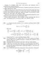
... = 50 and Nt = 50 0, so k = × 10−3 and h = 0.2, we found that err0 = 1 .5 × 10−3 for FTCS and err0 = 1.7 × 10⁻³ for BTCS With Crank– Nicolson we were able to reduce Nt to 50 , so k = × 10−2 , and ... = 0.63 1 .5 0 .5 −0 .5 −1 −1 .5 100 80 15 60 10 40 20 t x Fig 23 .5 FTCS solution on the heat equation (23.2), (23.3) and (23.4) with initial and boundary conditions (23 .5) Here N x = 14 and Nt = ... > 23.7 Show that Crank–Nicolson, (23.18), can be expressed as 2 − νδx U i+1 = + νδx U ij j 2 23.8 By analogy with (23.13) and (23. 15) , define the local accuracy for Crank–Nicolson and show that...
Ngày tải lên: 21/06/2014, 04:20

An Introduction to Financial Option Valuation_12 pptx
... 174, 1 75 ARCH, see autoregressive conditional heteroscedasticity Asian option, 192–194, 196 ask price, asset model continuous, 56 , 59 , 60 discrete, 54 , 55 , 60, 151 incremental, 56 mean, 56 , 60, ... 1 75, 182 liquidity, 94 log ratio, 48, 203, 210 lognormal distribution, 56 , 57 , 59 , 60, 66, 70, 118 London International Financial Futures and Options Exchange, 5, 1 35 London Stock Exchange, 50 ... option, 191 down-and-in call, 188, 189 down-and-in put, 190 down-and-out call, 187–189, 260–261, 2 65 down-and-out put, 190 drift, 54 , 1 05, 198 efficient market hypothesis, 45 46, 49, 51 , 52 , 54 ,...
Ngày tải lên: 21/06/2014, 04:20

An Introduction to Financial Option Valuation Mathematics Stochastics and Computation_1 doc
... Market values for IBM call and put options, for a range of strike prices and times to expiry 1.6 Notes and references 50 Call value 35 30 Asset price now 25 20 15 10 30 40 50 60 70 80 90 100 110 ... arguments to those above can be used to obtain simple upper and lower bounds on the values C and P of European call and put options To study the call option, consider two portfolios: π A : one call option ... price, both the call and the put option prices 80 40 60 150 100 50 Now Strike mths wks Tim e to 20 27 mths ry 15 mths 40 ex pi 10 exp i ry 27 mths 15 mths 150 100 Now 50 mths wks to Put 20 e Call...
Ngày tải lên: 21/06/2014, 07:20

An Introduction to Financial Option Valuation Mathematics Stochastics and Computation_4 docx
... Part II 2 .5 1 .5 0 .5 0 0.2 0.3 0.4 0 .5 0.6 0.7 0.8 0.9 0 .5 1 .5 2 .5 3 .5 4 .5 0.8 0.6 0.4 0.2 Fig 7.4 Upper picture: 50 discrete asset paths over [0, T ] with S0 = 1, µ = 0. 05, σ = 0 .5, T = and δt = ... S0 = 5, E = 4, T = 1, σ = 0.3 82 Black–Scholes PDE and formulas and r = 0. 05, we find, to four decimal places, d1 = 1.06 05, d2 = 0.76 05, N (d1 ) = 0. 855 5, N (d2 ) = 0.77 65, N (−d1 ) = 0.14 45, N ... the company and has many insights into the practical issues involved in collecting and analysing vast amounts of financial data EXERCISES 7.1 7.2 Confirm the results (7.4) and (7 .5) By analogy...
Ngày tải lên: 21/06/2014, 07:20

An Introduction to Financial Option Valuation Mathematics Stochastics and Computation_9 ppt
... 1.7983 1.7962 1.7962 177 18 .5 Optimal exercise boundary American put 1.82 1.8 15 1.81 1.8 05 1.8 1.7 95 50 100 150 200 250 M American put 1.79 85 1.798 1.79 75 1.797 1.79 65 1.796 200 220 240 260 280 ... Exercise 19.6 19 .5 Bermudan and shout options A Bermudan option differs from the corresponding American option in only one respect While the American option allows the holder to exercise at any time ... gives an approximate option price a M and an approximate 95% confidence interval ( 15. 5) For Asian options we could use the Riemann sum t N S j to approximate j=1 T the integral S(τ )dτ With an average...
Ngày tải lên: 21/06/2014, 07:20