numerical methods for parabolic equations

Numerical methods for maxwell equations
... Numerical Methods for Maxwell Equations Joachim Schăoberl SS05 Abstract The Maxwell equations describe the interaction of electric and magnetic ... required In this lecture we formulate the Maxwell equations, and discuss the finite element method to solve them Involved topics are partial differential equations, variational formulations, edge elements, ... elements, preconditioning, a posteriori error estimates Maxwell Equations In this chapter we formulate the Maxwell equations 1.1 The equations of the magnetic fields The involved field quantities
Ngày tải lên: 26/01/2022, 15:15

HIGH ORDER ACCURATE METHODS FOR MAXWELL EQUATIONS kashdan
... for compact high-order finite difference scheme Applied Numerical Analysis, 12:55–81, 1993 [13] J J Dongarra, I S Duff, D C Sornesen, and H A van der Vorst Numerical Linear Algebra for High-Performance ... Boston, MA, 1998 [20] D Givoli Numerical Methods for Problems in Infinite Domains Elsevier, Amsterdam, 1992 [21] S Goedecker and A Hoisie Performance Optimization of Numericaly Intensive Codes SIAM, ... dependent approach to solving the Maxwell equations This approach has the advantage that for explicit schemes no matrix inversion is necessary or for compact implicit methods only low dimension sparse
Ngày tải lên: 17/03/2014, 14:29

compact numerical methods for computers linear algebra and function minimisation 2ed - adam hilger
... 244 Fletcher-Reeves formula, 199 FMIN linear search program, 153 Ford B., 135 Formulae, Gauss-Jordan, 98 Forsythe, G E., 127, 153 FORTRAN, 10, 56, 63 Forward difference, 19 Forward-substitution, ... generalised, 104, 148 Matrix eigenvalues for polynomial roots, 148 Matrix form of linear equations, 19 Matrix inverse for linear equations, 24 275 Matrix iteration methods for function minimisation, 187 ... of numerical methods for design optimization Report No lJTME-TP7204 (Toronto, Ont.: Dept of Mechanical Engineering, Univ of Toronto) -1973 A comparison of numerical optimization methods for
Ngày tải lên: 31/03/2014, 15:02

Báo cáo hóa học: " Research Article On Comparison Principles for Parabolic Equations with Nonlocal Boundary Conditions" potx
... 1. Introduction The positivity of solutions for parabolic problems is the base of comparison principle which is important in monotonic methods used for these problems. Recently, Yin [1]de- veloped ... necessary for problems with lower regularity (see [3, Theorem 3.11] for problem with Dirichlet-type nonlocal boundary value). Moreover, in [7], an existence result for classical solutions of a parabolic ... Article ID 80929, 10 pages doi:10.1155/2007/80929 Research Article On Comparison Principles for Parabolic Equations with Nonlocal Boundary Conditions Yuandi Wang and Hamdi Zorgati Received 5 December
Ngày tải lên: 22/06/2014, 19:20

High resolution numerical methods for compressible multi fluid flows and their applications in simulations
... (1997) Volume-tracking methods for interfacial flow calculations International Journal for Numerical Methods in Fluids, 24:671–691 Rudman, M (1998) A volume-tracking method for incompressible multifluid ... (2008c) A piecewise parabolic method for barotropic and nonbarotropic two-fluid flows International Journal of Numerical Methods for Heat & Fluid Flow, 18(6):708–729 Zoldi, C A (2002) A numerical and ... finite element scheme for transient problems in CFD Computer Methods in Applied Mechanics and Engineering, 61:323–338 Ma, D J (2002) Study of high resolution numerical methods for compress- ible/incompressible
Ngày tải lên: 14/09/2015, 08:44
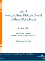
Introduction to Numerical Methods for Diferentia
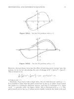
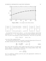
... to Numerical Methods for Differential and Differential Algebraic Equations TU Ilmenau , θ(0) = π4 ω(0) = Commonly, numerical methods are developed for systems of first order differential equations ... to Numerical Methods for Differential and Differential Algebraic Equations TU Ilmenau We us the forward-difference numerical approximation for F (uk ): F (u(k) ) = F (u(k) + ∆) − F (u(k) ) ∆ for ... l x˙ = − Numerical Methods of Ordinary Differential Equations Initial Value Problems (IVPs) Lecture Introduction1 to Numerical Methods for Differential and Differential Algebraic Equations TU
Ngày tải lên: 21/12/2016, 10:34

Mathematical theory and numerical methods for boseeinstein condensation
... 8.6 Numerical methods for computing ground states 8.7 Time splitting scheme for dynamics 8.8 Numerical results 8.9 Extensions in lower dimensions Mathematical theory and numerical methods for ... 113 113 114 115 118 MATHEMATICS AND NUMERICS FOR BEC 9.5 Numerical methods for computing ground states 9.6 Numerical methods for computing dynamics 9.7 Numerical results 10 Perspectives and challenges ... Simplified methods for symmetric potential and initial data 4.4 Error estimates for SIFD and CNFD 4.5 Error estimates for TSSP 4.6 Numerical results 4.7 Extension to damped Gross-Pitaevskii equations
Ngày tải lên: 11/06/2017, 14:46

Numerical methods for inverse problems
... Numerical Methods for Inverse Problems To my wife Elisabeth, to my children David and Jonathan Series Editor Nikolaos Limnios Numerical Methods for Inverse Problems Michel ... NABNER P., A NGERMANN L., Numerical Methods for Elliptic and Parabolic Partial Differential Equations, Springer Verlag, New York, 2003 [KRE 89] K RESS R., Linear Integral Equations, Springer, Berlin, ... 71, 106, 114, 193 D Numerical Methods for Inverse Problems, First Edition Michel Kern © ISTE Ltd 2016 Published by ISTE Ltd and John Wiley & Sons, Inc 214 Numerical Methods for Inverse Problems
Ngày tải lên: 14/05/2018, 15:40

Solution manual for applied numerical methods for engineers using MATLAB and c 1st edition by schilling
... Manual for Applied Numerical Methods for Engineers Using MATLAB and C 1st Edition Solution Manual for Applied Numerical Methods for Engineers Using MATLAB and C 1st Edition Solution Manual for ... Applied Numerical Methods for Engineers Using MATLAB and C 1st Edition Solution Manual for Applied Numerical Methods for Engineers Using MATLAB and C 1st Edition Solution Manual for Applied Numerical ... Numerical Methods for Engineers Using MATLAB and C 1st Edition Solution Manual for Applied Numerical Methods for Engineers Using MATLAB and C 1st Edition Solution Manual for Applied Numerical Methods
Ngày tải lên: 20/08/2020, 13:34

Introduction to numerical methods in differential equations ( 2007)
... ed 44 Knabner/Angermann: Numerical Methods for Elliptic and Parabolic Partial Differential Equations 45 Larsson/Thomée: Partial Differential Equations with Numerical Methods 46 Pedregal: Introduction ... and Queues 32 Durran: Numerical Methods for Wave Equations in Geophysical Fluids Dynamics 33 Thomas: Numerical Partial Differential Equations: Conservation Laws and Elliptic Equations 34 Chicone: ... Differential Equations Springer, New York, 2002 D R Durran Numerical Methods for Wave Equations in Geophysical Fluid Dynamics Springer, New York, 1998 L C Evans Partial Differential Equations American
Ngày tải lên: 07/09/2020, 11:20

Numerical methods for differential equations with distributional derivatives
... why we will consider numerical methods for solving this kind of differential equations However, the exact solution in hand can be used as benchmark to evaluate numerical methods In the following ... Please refer to [12] for more details Other than finite element method, in this paper, we will discuss an alternative numerical method to handle the equations with distributions For the purpose of ... this thesis, we will mainly consider the numerical method for differential equations with the delta distribution and its distributional derivatives Such equations have very strong physical backgrounds...
Ngày tải lên: 27/11/2015, 11:12

Numerical Methods for Ordinary Differential Equations Butcher Tableau doc
... Numerical Methods for Ordinary Differential Equations Numerical Methods for Ordinary Differential Equations, Second Edition J C Butcher © 2008 John Wiley & Sons, Ltd ISBN: 978-0-470-72335-7 Numerical ... in detail the design of efficient explicit methods for non-stiff xiv NUMERICAL METHODS FOR ORDINARY DIFFERENTIAL EQUATIONS problems For implicit methods for stiff problems, inexpensive implementation ... which Numerical Methods for Ordinary Differential Equations, Second Edition J C Butcher © 2008 John Wiley & Sons, Ltd ISBN: 978-0-470-72335-7 NUMERICAL METHODS FOR ORDINARY DIFFERENTIAL EQUATIONS...
Ngày tải lên: 27/06/2014, 08:20

Numerical Methods for Ordinary Differential Equations Numerical Methods pptx
... Numerical Methods for Ordinary Differential Equations Numerical Methods for Ordinary Differential Equations, Second Edition J C Butcher © 2008 John Wiley & Sons, Ltd ISBN: 978-0-470-72335-7 Numerical ... in detail the design of efficient explicit methods for non-stiff xiv NUMERICAL METHODS FOR ORDINARY DIFFERENTIAL EQUATIONS problems For implicit methods for stiff problems, inexpensive implementation ... which Numerical Methods for Ordinary Differential Equations, Second Edition J C Butcher © 2008 John Wiley & Sons, Ltd ISBN: 978-0-470-72335-7 NUMERICAL METHODS FOR ORDINARY DIFFERENTIAL EQUATIONS...
Ngày tải lên: 27/06/2014, 18:20

Numerical Methods for Ordinary Dierential Equations Episode 1 docx
... Numerical Methods for Ordinary Differential Equations Numerical Methods for Ordinary Differential Equations, Second Edition J C Butcher © 2008 John Wiley & Sons, Ltd ISBN: 978-0-470-72335-7 Numerical ... in detail the design of efficient explicit methods for non-stiff xiv NUMERICAL METHODS FOR ORDINARY DIFFERENTIAL EQUATIONS problems For implicit methods for stiff problems, inexpensive implementation ... which Numerical Methods for Ordinary Differential Equations, Second Edition J C Butcher © 2008 John Wiley & Sons, Ltd ISBN: 978-0-470-72335-7 NUMERICAL METHODS FOR ORDINARY DIFFERENTIAL EQUATIONS...
Ngày tải lên: 13/08/2014, 05:21
Numerical Methods for Ordinary Dierential Equations Episode 2 docx
... have Numerical Methods for Ordinary Differential Equations, Second Edition J C Butcher © 2008 John Wiley & Sons, Ltd ISBN: 978-0-470-72335-7 52 NUMERICAL METHODS FOR ORDINARY DIFFERENTIAL EQUATIONS ... Lotka–Volterra equations (106a), (106b) in the form given in Exercise 12.1 38 NUMERICAL METHODS FOR ORDINARY DIFFERENTIAL EQUATIONS 13 Difference Equation Problems 130 Introduction to difference equations ... given by 32 NUMERICAL METHODS FOR ORDINARY DIFFERENTIAL EQUATIONS 102 Figure 121(ii) 1+ √ 2+ √ 2 √ √ 1+ √ 10 Solution to neutral delay differential equation (121c) the formula for y (x) for x positive...
Ngày tải lên: 13/08/2014, 05:21
Numerical Methods for Ordinary Dierential Equations Episode 3 pot
... which of various alternative numerical methods should be used for a specific problem, or even for a large class of problems 56 NUMERICAL METHODS FOR ORDINARY DIFFERENTIAL EQUATIONS Table 201(II) h ... 12 12 −9 NUMERICAL METHODS FOR ORDINARY DIFFERENTIAL EQUATIONS 0.05 h 0.10 0.15 62 Figure 203(iii) x Stepsize h against x for the ‘mildly stiff’ problem (203a) with variable stepsize for T = 0.02 ... function, y, on [x0 , x] by the formula y(x) = y(xk−1 ) + (x − xk−1 )f (xk−1 , y(xk−1 )), x ∈ (xk−1 , xk ], (210b) 66 NUMERICAL METHODS FOR ORDINARY DIFFERENTIAL EQUATIONS for k = 1, 2, , n If we...
Ngày tải lên: 13/08/2014, 05:21

Numerical Methods for Ordinary Dierential Equations Episode 4 doc
... to converge for large stepsizes (not shown in the diagrams) This effect persisted for a larger range of stepsizes for PEC methods than was the case for PECE methods NUMERICAL METHODS FOR ORDINARY ... than for corresponding explicit NUMERICAL METHODS FOR ORDINARY DIFFERENTIAL EQUATIONS 10−6 10−4 104 −8 E 10 10 −10 10−4 Figure 239(ii) 10−3 h 10−2 Runge–Kutta methods with cost corrections methods ... criteria to derive Adams–Bashforth methods with p = k for k = 2, 3, 4, and Adams–Moulton methods with p = k + for k = 1, 2, For k = 4, the Taylor expansion of (241c) takes the form hy (xn )(1 − β0 −...
Ngày tải lên: 13/08/2014, 05:21

Numerical Methods for Ordinary Dierential Equations Episode 5 docx
... 124 NUMERICAL METHODS FOR ORDINARY DIFFERENTIAL EQUATIONS 262 Generalized linear multistep methods These methods, known also as hybrid methods or modified linear multistep methods, generalize ... by Numerical Methods for Ordinary Differential Equations, Second Edition J C Butcher © 2008 John Wiley & Sons, Ltd ISBN: 978-0-470-72335-7 138 NUMERICAL METHODS FOR ORDINARY DIFFERENTIAL EQUATIONS ... interpolation formula in the form y(xn−1 + ht) ≈ (1 + 2t)(1 − t)2 y(xn−1) + (3 − 2t)t2 y(xn ) + t(1 − t)2 hy (xn−1 ) − t2 (1 − t)hy (xn ) 132 NUMERICAL METHODS FOR ORDINARY DIFFERENTIAL EQUATIONS...
Ngày tải lên: 13/08/2014, 05:21

Numerical Methods for Ordinary Dierential Equations Episode 6 ppsx
... 1/γ(t3 ) For explicit methods, D(2) cannot hold, for similar reasons to the impossibility of C(2) For implicit methods D(s) is possible, as we shall see in Section 342 174 NUMERICAL METHODS FOR ORDINARY ... of the matrix A For i corresponding to a member of row k for k = 1, 2, , m, the only non-zero 190 NUMERICAL METHODS FOR ORDINARY DIFFERENTIAL EQUATIONS aij are for j = and for j corresponding ... 31.3 For an arbitrary Runge–Kutta method, find the order condition corresponding to the tree 170 NUMERICAL METHODS FOR ORDINARY DIFFERENTIAL EQUATIONS 32 Low Order Explicit Methods 320 Methods...
Ngày tải lên: 13/08/2014, 05:21
Numerical Methods for Ordinary Dierential Equations Episode 7 potx
... I formula, c1 = This formula is exact for polynomials of degree up to 2s − II For the Radau II formula, cs = This formula is exact for polynomials of degree up to 2s − III For the Lobatto formula, ... p + (333g) 204 NUMERICAL METHODS FOR ORDINARY DIFFERENTIAL EQUATIONS Proof For a given tree t, let Φ(t) denote the elementary weight for (333a) and Φ(t) the elementary weight for (333b) Because ... of degree 216 NUMERICAL METHODS FOR ORDINARY DIFFERENTIAL EQUATIONS ∗ less than n − A simple calculation shows that Q is orthogonal to Pk for ∗ k < n − Hence, (342f) follows except for the value...
Ngày tải lên: 13/08/2014, 05:21