methods for solving integral equations

Báo cáo hóa học: "Review Article T -Stability Approach to Variational Iteration Method for Solving Integral Equations" pot
... “Two methods for solving integral equations, ” Applied Mathematics and Computation, vol 77, no 1, pp 79–89, 1996 10 A M Wazwaz, “A reliable treatment for mixed Volterra-Fredholm integral equations, ” ... Fredholm integral equation of second kind in the general case, which reads b u x f x 1.4 K x, t u t dt, λ a where K x, t is the kernel of the integral equation There is a simple iteration formula for ... Dehghan, S M Vaezpour, and M Saravi, “The convergence of He’s variational iteration method for solving integral equations, ” Computers and Mathematics with Applications In press ...
Ngày tải lên: 21/06/2014, 20:20

Methods for solving inverse problems in mathematical physics prilepko, orlovskiy
... Problems for Equations Problems for Equations of Hyperbolic Type Inverse problems for x-hyperbolic systems Inverse problems for t-hyperbolic systems Inverse problems for hyperbolic equations ... Problems for Equations of Second Order Cauchy problem for semilinear hyperbolic equations Two-point inverse problems for equations of hyperbolic type Two-point inverse problems for equations ... inverse problems for mathematical physics equations, in particular, for parabolic equations, second order elliptic and hyperbolic equations, the systems of Navier-Stokes and Maxwell equations, symmetric...
Ngày tải lên: 17/03/2014, 14:30

hilbert space methods for partial differential equations - r. showalter
... Semigroups Parabolic Equations V Implicit Evolution Equations Introduction Regular Equations Pseudoparabolic Equations Degenerate Equations Examples ... so that j C0 j (x) for all x Rn , supp( j ) Gj , and j (x) = for x Fj LetS C0 (Rn ) be chosen with (x) n , supp( ) G for all x R fFj : j N g, and (x) P for x G = Finally, for each j , j N , ... Approximation of Evolution Equations Introduction Regular Equations Sobolev Equations Degenerate Equations Examples ...
Ngày tải lên: 31/03/2014, 15:56

Báo cáo hóa học: " Research Article Resolvent Iterative Methods for Solving System of Extended General Variational Inclusions" potx
... Noor, “Resolvent methods for solving a system of variational inclusions,” International Journal of Modern Physics B In press 27 M A Noor and K I Noor, “Resolvent methods for solving the system ... 0, for all n ≥ satisfies some suitable conditions For suitable and appropriate choice of the operators T1 , T2 , A, g, h, g1 and spaces, one can obtain a wide class of iterative methods for solving ... the required result This equivalent formulation is used to suggest and analyze an iterative method for solving 2.1 To so, one rewrite 3.3 in the following form: x∗ − an x∗ y∗ an x∗ − g1 x∗ y...
Ngày tải lên: 21/06/2014, 06:20
Báo cáo hóa học: " Research Article Some Iterative Methods for Solving Equilibrium Problems and Optimization Problems" potx
... Preliminaries For solving the equilibrium problem for a bifunction F : C × C → R, let us assume that F satisfies the following conditions: A1 F x, x for all x ∈ C; A2 F is monotone, that is, F x, y A3 for ... for all x ∈ C, for a constant κ > 1; then, T is relaxed μ, ν -cocoercive and Lipschitz continuous Especially, T is ν-strong monotone Proof Since T x κx, for all x ∈ C, we have T : C → C For for ... method for solving the variational inequality 1.2 For a given u0 ∈ C, wn un PC un − λAun , PC wn − λAwn , n 0, 1, 2, , 1.7 which is also known as the modified double-projection method For the...
Ngày tải lên: 21/06/2014, 07:20

Báo cáo hóa học: " Research Article Existence Principle for Advanced Integral Equations on Semiline" pot
... ≤ C for any k ∈ N, where Ln = 2n+1 n−1 k(s)ds Then there exists at least one solution x ∈ C(R+ ,E) of the integral equation (2.1) Proof For the proof we use Theorem 1.3 Let X = C(R+ ,E) For each ... has a fixed point Therefore, all the assumptions of Theorem 1.3 are satisfied Now the conclusion follows from Theorem 1.3 Other existence results for integral and differential equations established ... Gordon and Breach Science, Amsterdam, The Netherlands, 2001 [7] A Chis, “Continuation methods for integral equations in locally convex spaces,” Studia Univer¸ sitatis Babes-Bolyai Mathematica,...
Ngày tải lên: 22/06/2014, 19:20

Numerical Methods for Ordinary Differential Equations Butcher Tableau doc
... in detail the design of efficient explicit methods for non-stiff xiv NUMERICAL METHODS FOR ORDINARY DIFFERENTIAL EQUATIONS problems For implicit methods for stiff problems, inexpensive implementation ... Numerical Methods for Ordinary Differential Equations Numerical Methods for Ordinary Differential Equations, Second Edition J C Butcher © 2008 John Wiley & Sons, Ltd ISBN: 978-0-470-72335-7 Numerical Methods ... functions on [0, 1] for which u(0) = u(1) = dx2 The eigenfunctions for the continuous problem are of the form sin(kπx), for 10 NUMERICAL METHODS FOR ORDINARY DIFFERENTIAL EQUATIONS k = 1, 2,...
Ngày tải lên: 27/06/2014, 08:20

Numerical Methods for Ordinary Dierential Equations Episode 1 docx
... in detail the design of efficient explicit methods for non-stiff xiv NUMERICAL METHODS FOR ORDINARY DIFFERENTIAL EQUATIONS problems For implicit methods for stiff problems, inexpensive implementation ... Numerical Methods for Ordinary Differential Equations Numerical Methods for Ordinary Differential Equations, Second Edition J C Butcher © 2008 John Wiley & Sons, Ltd ISBN: 978-0-470-72335-7 Numerical Methods ... functions on [0, 1] for which u(0) = u(1) = dx2 The eigenfunctions for the continuous problem are of the form sin(kπx), for 10 NUMERICAL METHODS FOR ORDINARY DIFFERENTIAL EQUATIONS k = 1, 2,...
Ngày tải lên: 13/08/2014, 05:21
Numerical Methods for Ordinary Dierential Equations Episode 2 docx
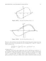
... by 32 NUMERICAL METHODS FOR ORDINARY DIFFERENTIAL EQUATIONS 102 Figure 121(ii) 1+ √ 2+ √ 2 √ √ 1+ √ 10 Solution to neutral delay differential equation (121c) the formula for y (x) for x positive ... Lotka–Volterra equations (106a), (106b) in the form given in Exercise 12.1 38 NUMERICAL METHODS FOR ORDINARY DIFFERENTIAL EQUATIONS 13 Difference Equation Problems 130 Introduction to difference equations ... matrix −2 , (131b) suggests that we can look for solutions for the original formulation in the form λn without transforming to the matrix–vector formulation Substitute this trial solution into...
Ngày tải lên: 13/08/2014, 05:21
Numerical Methods for Ordinary Dierential Equations Episode 3 pot
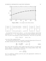
... various alternative numerical methods should be used for a specific problem, or even for a large class of problems 56 NUMERICAL METHODS FOR ORDINARY DIFFERENTIAL EQUATIONS Table 201(II) h π 200 ... ‘convergence’ In searching for other numerical methods that are suitable for solving initial value problems, attention is usually limited to convergent methods The reason for this is clear: a non-convergent ... function, y, on [x0 , x] by the formula y(x) = y(xk−1 ) + (x − xk−1 )f (xk−1 , y(xk−1 )), x ∈ (xk−1 , xk ], (210b) 66 NUMERICAL METHODS FOR ORDINARY DIFFERENTIAL EQUATIONS for k = 1, 2, , n If we...
Ngày tải lên: 13/08/2014, 05:21

Numerical Methods for Ordinary Dierential Equations Episode 4 doc
... diagrams) This effect persisted for a larger range of stepsizes for PEC methods than was the case for PECE methods NUMERICAL METHODS FOR ORDINARY DIFFERENTIAL EQUATIONS 10−6 10−4 114 10−8 E 10−10 ... values for the Adams– Bashforth methods are given in Table 244(I) and for the Adams–Moulton methods in Table 244(II) The Adams methods are usually implemented in ‘predictor–corrector’ form That ... criteria to derive Adams–Bashforth methods with p = k for k = 2, 3, 4, and Adams–Moulton methods with p = k + for k = 1, 2, For k = 4, the Taylor expansion of (241c) takes the form hy (xn )(1 − β0 −...
Ngày tải lên: 13/08/2014, 05:21

Numerical Methods for Ordinary Dierential Equations Episode 5 docx
... 124 NUMERICAL METHODS FOR ORDINARY DIFFERENTIAL EQUATIONS 262 Generalized linear multistep methods These methods, known also as hybrid methods or modified linear multistep methods, generalize ... Numerical Methods for Ordinary Differential Equations, Second Edition J C Butcher © 2008 John Wiley & Sons, Ltd ISBN: 978-0-470-72335-7 138 NUMERICAL METHODS FOR ORDINARY DIFFERENTIAL EQUATIONS ... −1 1 0 1 2 1 1 6 3 126 NUMERICAL METHODS FOR ORDINARY DIFFERENTIAL EQUATIONS The second order Adams–Bashforth and Adams–Moulton and PECE methods based on these are, respectively, ...
Ngày tải lên: 13/08/2014, 05:21

Numerical Methods for Ordinary Dierential Equations Episode 6 ppsx
... 1/γ(t3 ) For explicit methods, D(2) cannot hold, for similar reasons to the impossibility of C(2) For implicit methods D(s) is possible, as we shall see in Section 342 174 NUMERICAL METHODS FOR ORDINARY ... of the matrix A For i corresponding to a member of row k for k = 1, 2, , m, the only non-zero 190 NUMERICAL METHODS FOR ORDINARY DIFFERENTIAL EQUATIONS aij are for j = and for j corresponding ... 31.3 For an arbitrary Runge–Kutta method, find the order condition corresponding to the tree 170 NUMERICAL METHODS FOR ORDINARY DIFFERENTIAL EQUATIONS 32 Low Order Explicit Methods 320 Methods...
Ngày tải lên: 13/08/2014, 05:21
Numerical Methods for Ordinary Dierential Equations Episode 7 potx
... I formula, c1 = This formula is exact for polynomials of degree up to 2s − II For the Radau II formula, cs = This formula is exact for polynomials of degree up to 2s − III For the Lobatto formula, ... (333g) 204 NUMERICAL METHODS FOR ORDINARY DIFFERENTIAL EQUATIONS Proof For a given tree t, let Φ(t) denote the elementary weight for (333a) and Φ(t) the elementary weight for (333b) Because the ... c1 = 0, cs = This formula is exact for polynomials of degree up to 2s − Furthermore, for each of the three quadrature formulae, ci ∈ [0, 1], for i = 1, 2, , s, and bi > 0, for i = 1, 2, ...
Ngày tải lên: 13/08/2014, 05:21

Numerical Methods for Ordinary Dierential Equations Episode 8 ppsx
... 12 36 For E(y) ≥ 0, for all y > 0, it is necessary and sufficient for A-stability that λ ∈ [ , λ], where λ ≈ 1.0685790213 is a zero of the coefficient of y in E(y) For 262 NUMERICAL METHODS FOR ORDINARY ... These include the Gauss methods e and the Radau IA and IIA methods as well as the Lobatto IIIC methods A corollary is that the Radau IA and IIA methods and the Lobatto IIIC methods are L-stable ... NUMERICAL METHODS FOR ORDINARY DIFFERENTIAL EQUATIONS Because θ cannot leave the interval [0, π], then for w to remain real, y is bounded as z → ∞ Furthermore, w → ∞ implies that x → −∞ The result for...
Ngày tải lên: 13/08/2014, 05:21

Numerical Methods for Ordinary Dierential Equations Episode 9 ppsx
... Runge–Kutta methods exist for which A is lower triangular? 280 NUMERICAL METHODS FOR ORDINARY DIFFERENTIAL EQUATIONS 38 Algebraic Properties of Runge–Kutta Methods 380 Motivation For any specific ... signs, where possible, and a preference for methods in which the ci lie in [0, 1] We illustrate these ideas for the case p = and s = 3, for which the general form for a method would be √ √ √ λ(2 − ... then the sub-forest induced by V is the forest (V , E), where E is the intersection of V × V and E A special 288 NUMERICAL METHODS FOR ORDINARY DIFFERENTIAL EQUATIONS case is when a sub-forest (V...
Ngày tải lên: 13/08/2014, 05:21

Numerical Methods for Ordinary Dierential Equations Episode 10 pot
... therefore over several steps 322 NUMERICAL METHODS FOR ORDINARY DIFFERENTIAL EQUATIONS 405 Necessity of conditions for convergence We formally prove that stability and consistency are necessary for ... Numerical Methods for Ordinary Differential Equations, Second Edition J C Butcher © 2008 John Wiley & Sons, Ltd ISBN: 978-0-470-72335-7 318 NUMERICAL METHODS FOR ORDINARY DIFFERENTIAL EQUATIONS ... method For a one-stage method, the evaluation technique is also similar for backward difference methods and for Runge–Kutta and general linear methods that have a lower triangular coefficient matrix For...
Ngày tải lên: 13/08/2014, 05:21

Numerical Methods for Ordinary Dierential Equations Episode 11 pptx
... variable order formulation It is natural to make a comparison between implementation techniques for Runge–Kutta methods and for linear multistep methods Unlike for explicit Runge–Kutta methods, interpolation ... method The first example is for the second order Adams–Bashforth method (430a) for which (431c) takes the form w→ − w−1 − w−2 −1 2w For w = exp(iθ) and θ ∈ [0, 2π], for points on the unit circle, ... this test in Subsection 433 346 NUMERICAL METHODS FOR ORDINARY DIFFERENTIAL EQUATIONS Algorithm 432α Boundary locus method for low order Adams–Bashforth methods % Second order % -w = exp(i*linspace(0,2*pi));...
Ngày tải lên: 13/08/2014, 05:21

Numerical Methods for Ordinary Dierential Equations Episode 12 pptx
... Adams–Bashforth method to variable stepsize 46.2 How should the formulation of Subsection 461 be modified to represent Adams–Bashforth methods? Chapter General Linear Methods 50 Representing Methods ... Numerical Methods for Ordinary Differential Equations, Second Edition J C Butcher © 2008 John Wiley & Sons, Ltd ISBN: 978-0-470-72335-7 374 NUMERICAL METHODS FOR ORDINARY DIFFERENTIAL EQUATIONS ... could be rewritten to produce formulae for the stages in the form Y = hAF + U y [n−1] = hAF + U T −1 z [n−1] (501a) The formula for y [n] = hBF + V y [n−1] , when transformed to give the value of...
Ngày tải lên: 13/08/2014, 05:21

Numerical Methods for Ordinary Dierential Equations Episode 13 pps
... given by Exercise 53.1 420 NUMERICAL METHODS FOR ORDINARY DIFFERENTIAL EQUATIONS 54 Methods with Runge–Kutta stability 540 Design criteria for general linear methods We consider some of the structural ... NUMERICAL METHODS FOR ORDINARY DIFFERENTIAL EQUATIONS stability properties that are usually superior to those of alternative methods For example, A-stability is inconsistent with high order for linear ... method based on several assumptions on the form of the method The original formulation for stiff methods was given in Butcher (2001) and for non-stiff methods in Wright (2002) In Butcher and Wright...
Ngày tải lên: 13/08/2014, 05:21