linear systems of two secondorder partial differential equations

Tài liệu Đề tài " Isomonodromy transformations of linear systems of difference equations" pptx
... deformations of two types: continuous ones, when x i move in the complex plane and B i = B i (x) form a solution of a sys- tem of partial differential equations called Schlesinger equations, and ... equal to I. The proof of uniqueness is complete. To prove the existence we note, first of all, that it suffices to provide a proof if one of the κ i ’s is equal to ±1 and one of the δ j ’s is equal ... for all k ∈ Z. The proof of the first part of Theorem 4.9 is complete. In order to prove Theorem 4.9(ii), we need to compare the first and the third factors of the two sides of (4.7). The first factors...
Ngày tải lên: 14/02/2014, 17:20
Báo cáo y học: "Modelling of oedemous limbs and venous ulcers using partial differential equations" pdf
Ngày tải lên: 13/08/2014, 23:20

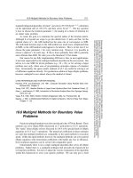
Partial Differential Equations part 1
... 19. Partial Differential Equations 19.0 Introduction The numerical treatment of partial differential equations is, by itself, a vast subject. Partial differential equations are at the heart of ... entiresecond volume of Numerical Recipes dealing with partial differential equations alone. (The references [1-4] provide, of course, available alternatives.) In most mathematics books, partial differential equations ... the solutionof large numbers of simultaneous algebraic equations. When such equations are nonlinear, they are usually solved by linearization and iteration; so without much loss of generality...
Ngày tải lên: 28/10/2013, 22:15

Partial Differential Equations part 2
... points two- step Lax Wendroff Figure 19.1.7. Representation of the two- step Lax-Wendroff differencing scheme. Two halfstep points (⊗) are calculated by the Lax method. These, plus one of the original ... set of two first-order equations ∂r ∂t = v ∂s ∂x ∂s ∂t = v ∂r ∂x (19.1.3) where r ≡ v ∂u ∂x s ≡ ∂u ∂t (19.1.4) In this case r and s become the two components of u, and the flux is given by the linear ... third type of error is one associated with nonlinear hyperbolic equations and is therefore sometimes called nonlinearinstability. For example, a piece of the Euler or Navier-Stokes equations for...
Ngày tải lên: 07/11/2013, 19:15

Tài liệu Partial Differential Equations part 3 pptx
... (19.2.22) with n → n +1leaves us with a nasty set of coupled nonlinear equations to solve at each timestep. Often there is an easier way: If the form of D(u) allows us to integrate dz = D(u)du (19.2.23) analytically ... evolve through of order λ 2 /(∆x) 2 steps before things start to happen on the scale of interest. This number of steps is usually prohibitive. We must therefore find a stable way of taking timesteps ... amplitudes, so that the evolution of the larger-scale features of interest takes place superposed with a kind of “frozen in” (though fluctuating) background of small-scale stuff. This answer gives...
Ngày tải lên: 15/12/2013, 04:15
Tài liệu Partial Differential Equations part 4 ppt
... value problems (elliptic equations, for example) reduce to solving large sparse linear systems of the form A· u = b (19.4.1) either once, for boundary value equations that are linear, or iteratively, ... ∆t) ··· u n+1 = U m (u n+(m−1)/m , ∆t) (19.3.20) 854 Chapter 19. Partial Differential Equations Sample page from NUMERICAL RECIPES IN C: THE ART OF SCIENTIFIC COMPUTING (ISBN 0-521-43108-5) Copyright (C) ... 1977, Numerical Methods for Partial Differential Equations , 2nd ed. (New York: Academic Press), Chapter 2. Goldberg, A., Schey, H.M., and Schwartz, J.L. 1967, American Journal of Physics , vol. 35, pp....
Ngày tải lên: 15/12/2013, 04:15
Tài liệu Partial Differential Equations part 5 ppt
... level of CR, we have reduced the number of equations by a factor of two. Since the resulting equations are of the same form as the original equation, we can repeat the process. Taking the number of ... problems (elliptic equations, for example) reduce to solving large sparse linear systems of the form A · u = b (19.4.1) either once, for boundary value equations that are linear, or iteratively, ... solve the tridiagonal equations by the usual algorithm in the other dimension) gives about a factor of two gain in speed. The optimal FACR with r =2gives another factor of two gain in speed. CITED...
Ngày tải lên: 15/12/2013, 04:15
Tài liệu Partial Differential Equations part 6 doc
... ease of programming outweighs expense of computer time. Occasionally, the sparse matrix methods of Đ2.7 are useful for solving a set of difference equations directly. For production solution of ... solve the tridiagonal equations by the usual algorithm in the other dimension) gives about a factor of two gain in speed. The optimal FACR with r =2gives another factor of two gain in speed. CITED ... America). The beauty of Chebyshev acceleration is that the norm of the error always decreases with each iteration. (This is the norm of the actual error in u j,l . The norm of the residual ξ j,l need...
Ngày tải lên: 15/12/2013, 04:15
Tài liệu Partial Differential Equations part 7 doc
... ease of programming outweighs expense of computer time. Occasionally, the sparse matrix methods of Đ2.7 are useful for solving a set of difference equations directly. For production solution of ... solution of it by introducing an even coarser grid and using the two- grid iteration method. If the convergence factor of the two- grid method is small enough, we will need only a few steps of this ... iteration of a multigrid method, from finest grid to coarser grids and back to finest grid again, is called a cycle. The exact structure of a cycle depends on the value of γ, the number of two- grid...
Ngày tải lên: 24/12/2013, 12:16

Functional analysis sobolev spaces and partial differential equations
... ∈ E. Proof of Corollary 2.8. Apply Corollary 2.7 with E = (E, 1 ), F = (E, 2 ), and T = I. Proof of Theorem 2.6. We split the argument into two steps: Step 1. Assume that T is a linear surjective ... ∈ E ;p(x) < 1}.(10) Proof of Lemma 1.2. It is obvious that (1) holds. Proof of (9). Let r>0 be such that B(0,r) ⊂ C; we clearly have p(x) ≤ 1 r x∀x ∈ E. Proof of (10). First, suppose that ... Sobolev Spaces and Partial Differential Equations, DOI 10.1007/978-0-387-70914-7_2, â Springer Science+Business Media, LLC 2011 Haim Brezis Distinguished Professor Department of Mathematics Rutgers...
Ngày tải lên: 04/02/2014, 11:10

Tài liệu AN INTRODUCTION TO PARTIAL DIFFERENTIAL EQUATIONS ppt
... Such equations are often called semilinear. r Scalar equations versus systems of equations A single PDE with just one unknown function is called a scalar equation. In contrast, a set of m equations ... of the gradient of u. While (1.3) is nonlinear, it is still linear as a function of the highest-order derivative. Such a nonlinearity is called quasilinear.On the other hand in (1.2) the nonlinearity ... computation of the Jacobian at points located on the initial curve , using 24 First-order equations 2.2 Quasilinear equations We consider first a special class of nonlinear equations where the nonlinearity...
Ngày tải lên: 16/02/2014, 15:20

Tài liệu Boundary Value Problems, Sixth Edition: and Partial Differential Equations pptx
... kinds of linear, homogeneous equations. Later, we will be using the same principle on partial differential equations. To be able to satisfy an unrestricted initial condition, we need two linearly ... the general solution of the differential equation. Chapter 0 Ordinary Differential Equations 3 Principle of Superposition. If u 1 (t) and u 2 (t) are solutions of the same linear homogeneous equation ... follow the derivations of the heat and wave equations. The principal objective of the book is solving boundary value problems involving partial differential equations. Separation of variables receives...
Ngày tải lên: 17/02/2014, 14:20

Partial Differential Equations and Fluid Mechanics doc
... such as blood) are of comparable density, then assigning the notion of the ratio of the density of the reactant to the total density would not be appropriate as the balance of linear momentum for ... consequence of the relative velocity between the two fluids, acting on the fluids. Bridges & Rajagopal (2006) associate the concentration with the ratio of the density of the reactant to the sum of ... understand the influence of geometry of the flow and roughness of the boundary (as measured by h ) on the behaviour of the fluid. 1.4 Time-dependent driving: dimension of the pullback attractor In...
Ngày tải lên: 14/03/2014, 10:20

Entropy and partial differential equations evans l c
... = ∂E ∂V T . Proof. 1. Think of E as a function of T,V ; that is, E = E(S(T,V ),V), where S(T,V ) means S as a function of T,V . Then ∂E ∂T V = ∂E ∂S ∂S ∂T V = T ∂S ∂T V = C V . Likewise, think of ... process ∆ consisting of “ ˜ Γ followed by the reversal of Γ”. Then ∆ would absorb Q = −( ˜ Q − − Q − ) > 0 units of heat at the lower temperature T 1 and emit the same Q units of heat at the higher ... C 1 parameterization of the graph of V = V (T ) gives an adiabatic path. b. The First Law, existence of E We turn now to our basic task, building E, S for our fluid system. The existence of these quantities...
Ngày tải lên: 17/03/2014, 14:29
harmonic analysis and partial differential equations - b. dahlberg, c. kenig
Ngày tải lên: 31/03/2014, 15:16

hilbert space methods for partial differential equations - r. showalter
Ngày tải lên: 31/03/2014, 15:56
introduction to partial differential equations - a computational approach - a. tveito, r. winther
Ngày tải lên: 31/03/2014, 15:56


partial differential equations and the finite element method - pave1 solin
Ngày tải lên: 31/03/2014, 15:57

partial differential equations, (ma3132 lecture notes) - b. neta (
Ngày tải lên: 31/03/2014, 15:57