Electromagnetic Waves and Antennas combined - Chapter 5 ppt
Electromagnetic Waves and Antennas combined - Chapter 5 ppt
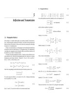
... quarter- wave, (b) both layers are half-wave, (c) layer-1 is quarter- and layer-2 half-wave, and (d) layer-1 is half- and layer-2 quarter-wave. Show that the reflection coefficient at interface-1 is ... relationships Eq. (5. 2.8), it is easily verified that Eq. (5. 2.13) is equivalent to the matching matrix equations (5. 2.3) and (5. 2.4). 5. 3. Reflected and Transmitted Power 159 5....
Ngày tải lên: 13/08/2014, 02:20
Electromagnetic Waves and Antennas combined - Chapter 3 ppt
... numeri- cally is equal to the phase of the complex number (1 + j)F(1/ √ 2BT). −20 − 15 −10 5 0 5 10 15 20 −1 .5 −1 −0 .5 0 0 .5 1 1 .5 time, t envelope FM pulse, T = 30, B = 4, f 0 = 0 −20 − 15 −10 5 ... 0 −20 − 15 −10 5 0 5 10 15 20 −1 .5 −1 −0 .5 0 0 .5 1 1 .5 time, t real part FM pulse, T = 30, B = 4, f 0 = 0 Fig. 3.12.1 Example graphs for Problem 3.13. −20 − 15 −1...
Ngày tải lên: 13/08/2014, 02:20

Electromagnetic Waves and Antennas combined - Chapter 14 ppt
... C −1 .5 −1 −0 .5 0 0 .5 1 1 .5 −1 .5 −1 −0 .5 0 0 .5 1 1 .5 t = 0 −1 .5 −1 −0 .5 0 0 .5 1 1 .5 −1 .5 −1 −0 .5 0 0 .5 1 1 .5 t = T /8 −1 .5 −1 −0 .5 0 0 .5 1 1 .5 −1 .5 −1 −0 .5 0 0 .5 1 1 .5 t = T /4 −1 .5 −1 −0 .5 0 ... discussed in Sec. 14.10. The near-field, non-radiating, terms in (14 .5. 5) that drop faster than 1 /r are im- portant in the new area of near-field o...
Ngày tải lên: 13/08/2014, 02:20

Electromagnetic Waves and Antennas combined - Chapter 15 ppt
... typically e a = 0 .55 –0 . 65. Combining Eqs. ( 15. 3 .5) and ( 15. 3.8), we obtain: G max = e a πd λ 2 ( 15. 3.9) Antennas fall into two classes: fixed-area antennas, such as dish antennas, for which A ... terms of G and f. 610 15. Transmitting and Receiving Antennas The beamwidth of a dish antenna can be estimated by combining the approximate ex- pression ( 15. 2.20) with...
Ngày tải lên: 13/08/2014, 02:20

Electromagnetic Waves and Antennas combined - Chapter 17 pptx
... the 3-dB and first-null widths in radians and degrees: Δθ 3dB = 0 .51 44 λ a = 29.47 o λ a ,Δθ null = 1.22 λ a = 70 o λ a (17.9 .5) The 3-dB angle is θ 3dB = Δθ 3dB /2 = 0. 257 2λ/a = 14.74 o λ/a and ... v x v y -plane: v 2 x +v 2 y ≤ a 2 λ 2 (17.9.4) The mainlobe/sidelobe characteristics of f(θ) are as follows. The 3-dB wavenumber is u = 0. 257 2 and the 3-dB width in u-space is Δu =...
Ngày tải lên: 13/08/2014, 02:20
Electromagnetic Waves and Antennas combined - Chapter 1 pps
... plane waves propagating in dielectrics, conductors, and birefringent me- dia, (b) guided waves propagating in hollow waveguides, transmission lines, and optical fibers, and (c) propagating waves ... current in the right-hand side of Amp ` ere’s law and accounts for both conducting and dielectric losses. The time-averaged version of Poynt- ing’s theorem is discussed in Problem 1...
Ngày tải lên: 13/08/2014, 02:20
Electromagnetic Waves and Antennas combined - Chapter 2 potx
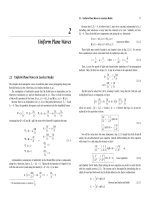
... 2π(2. 45 10 9 )/(3×10 8 )= 51 .31 rad/m. Using k c = ω √ μ 0 c = k 0 c / 0 , we calculate the wavenumbers: k c = β − jα = 51 .31 4 −j = 51 .31(2.02 − 0.25j)= 103.41 −12.73j m −1 k c = β − jα = 51 .31 45 −15j = 51 .31(6.80 ... other. Examples of such waves are the evanescent waves in total internal reflection, various guided-wave problems, such as surface waves, leaky wa...
Ngày tải lên: 13/08/2014, 02:20
Electromagnetic Waves and Antennas combined - Chapter 4 pdf
... D x = 0 and E x /E y =−j 2 / 1 . Eq. (4.7.4) and the results of Problem 4.14 lead to the so-called Appleton-Hartree equations for describing plasma waves in a magnetic field [720–724]. 4. 15 A uniform ... appropriate linear combinations. For example, we define the right-polarized (forward-moving) and left-polarized (backward- moving) waves for the {E + ,H + } case: E R+ = 1 2 E +...
Ngày tải lên: 13/08/2014, 02:20
Electromagnetic Waves and Antennas combined - Chapter 6 potx
... -0 .2000 -0 .4000 0 .50 00 A= 1.0000 1.0000 1.0000 1.0000 -0 .1000 -0 .1200 -0 .2000 0 -0 .0640 -0 .1000 0 0 -0 . 050 0000 B= -0 .1000 -0 .2000 -0 .4000 0 .50 00 -0 .1880 -0 .3600 0 .50 00 0 -0 . 350 0 0 .50 00 0 0 0 .50 00000 n= 1.0000 ... N 3 = 9 and N 2 = 10. Fig. 6 .5. 4 shows the case of four FPRs (case 4 in Eq. (6 .5. 1).) Again, a symmetric a...
Ngày tải lên: 13/08/2014, 02:20
Electromagnetic Waves and Antennas combined - Chapter 7 potx
... 54 .623 o and θ = 48.624 o . The rhomb could just as easily be designed with the second value of θ. For n = 1 .50 , we find the angles θ = 53 . 258 o and 50 .229 o . For n = 1 .52 , we have θ = 55 . 458 o and ... −sin 2 θ c sin 2 θ = tan π 8 (7 .5. 8) However, the two-step process is computationally more convenient. For n = 1 .51 , we find the two roots of Eq. (7 .5. 6): x = 0.8...
Ngày tải lên: 13/08/2014, 02:20