David G. Luenberger, Yinyu Ye - Linear and Nonlinear Programming International Series Episode 1 Part 2 ppsx
David G. Luenberger, Yinyu Ye - Linear and Nonlinear Programming International Series Episode 1 Part 1 doc
... Sensitivity 339 11 .8. Inequality Constraints 3 41 11. 9. Zero-Order Conditions and Lagrange Multipliers 346 11 .10 . Summary 353 11 .11 . Exercises 354 Chapter 12 . Primal Methods 359 12 .1. Advantage of ... 3 21 11. 2. Tangent Plane 323 11 .3. First-Order Necessary Conditions (Equality Constraints) 326 11 .4. Examples 327 11 .5. Second-Order Conditions 333 11 .6. Eigenvalues in...
Ngày tải lên: 06/08/2014, 15:20
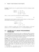
David G. Luenberger, Yinyu Ye - Linear and Nonlinear Programming International Series Episode 1 Part 2 ppsx
... equations x 1 + x 2 −x 3 = 5 2x 1 −3x 2 +x 3 = 3 −x 1 +2x 2 −x 3 = 1 To obtain an original basis, we form the augmented tableau e 1 e 2 e 3 a 1 a 2 a 3 b 10 0 1 1 15 010 2 313 0 01 12 1 1 and replace e 1 by ... obtain x 1 x 2 x 3 x 4 x 5 x 6 3/ 51/ 5 010 2/ 518 /5 2/ 5 1/ 50 01 3/57/5 1/ 53/ 510 0 1/ 5 1/ 5 Continuing, there results x 1 x 2 x 3...
Ngày tải lên: 06/08/2014, 15:20
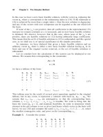
David G. Luenberger, Yinyu Ye - Linear and Nonlinear Programming International Series Episode 1 Part 3 ppsx
... sake of safety. 54 Chapter 3 The Simplex Method x 2 x 3 x 4 x 5 x 6 x 7 b 1 10 1 10 1 12 10 11 2 1 − 210 20−2 Second tableau—phase I 01 11 01 3 12 10 11 2 00 00 11 0 Final tableau—phase I Now ... problem x 2 x 3 x 4 x 5 b 01 11 3 12 10 2 c T 23 11 14 Initial tableau—phase II Transforming the last row appropriately we proceed with: 01 11 3 1 2 10 2 0 −220− 21 Fi...
Ngày tải lên: 06/08/2014, 15:20

David G. Luenberger, Yinyu Ye - Linear and Nonlinear Programming International Series Episode 1 Part 4 doc
... and new as follows. Variable B 1 Value s 1 1 10 012 2 0 1/ 2 0 1 1/2 0 1 0 1/ 2 1 1 1/ 2 1 2 0 0 0 1 1/2 0 s 1 10−2 −20 2 0 1/ 2 0 1 1/2 3 0 1/ 2 1 1 1/ 2 3 0 0 011 T = 0 4 ... −3000 1 1 1/ 2 1/ 2 0 2 10 1 11 2 30 12 0 8 3/2 1 0 1 1/ 21 10 1 11 2 20 01 110 The optimal solution is x 1 =0, x 2 =1, x 3 =2. The corresponding dual progr...
Ngày tải lên: 06/08/2014, 15:20
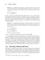
David G. Luenberger, Yinyu Ye - Linear and Nonlinear Programming International Series Episode 1 Part 5 docx
... row. a 1 a 2 a 3 ··b 1 12 10 3 213 0 15 −3 −2 50 0−8 1/ 203/2 ··· Second tableau Minimizing the new associated restricted primal by pivoting as indicated we obtain a 1 a 2 a 3 ··b 11 210 3 10 1 11 2 10 12 0−2 1/ 203/2 ... tableau: a 1 a 2 a 3 ··b 011 2 11 10 1 11 2 00 011 0 0 01 ·· Final tableau ∗ 4.7 Reduction of Linear Inequalities 10 1 By subtracting the second equati...
Ngày tải lên: 06/08/2014, 15:20
David G. Luenberger, Yinyu Ye - Linear and Nonlinear Programming International Series Episode 1 Part 6 pptx
... +1 = 1+ 1 m 2 1 m 1 /2 1 1 m +1 < exp 1 2m +1 − 1 m +1 =exp − 1 2m +1 Convergence The ellipsoid method is initiated by selecting y 0 and R such that condition (A1) ... S 1 we have d x +S 1 Xd s =S 1 1−x Then, premultiplying by A and using Ad x =0, we have AS 1 Xd s =AS 1 1−Ax =AS 1 1−b Using d s =−A T d y we have AS 1 XA T...
Ngày tải lên: 06/08/2014, 15:20
David G. Luenberger, Yinyu Ye - Linear and Nonlinear Programming International Series Episode 1 Part 7 pps
... constraint equations in standard form: x 11 +x 12 +···+x 1n =a 1 x 21 +x 22 +···+x 2n =a 2 x m1 +x m2 +···+x mn =a m x 11 +x 21 x m1 =b 1 x 12 + x 22 + x m2 =b 2 x 1n + x 2n + x mn =b n (3) The ... [V3], and Wright [W8]. 16 2 Chapter 6 Transportation and Network Flow Problems 1 2 3 4 (1, 2) (1, 4) (2, 3) (2, 4) (4, 2) 11 11 1 1 1 1 11 Table 6 .1 In...
Ngày tải lên: 06/08/2014, 15:20
David G. Luenberger, Yinyu Ye - Linear and Nonlinear Programming International Series Episode 1 Part 8 pdf
... 1) (3, 2) (3, 1) (1, 2) (5, 1) 2 3 3 4 5 6 2 2 2 1 1 1 1 1 1 1 1 1 1 1 (–, ∞) (2, 1) (1, 1) (5, 1) 2 4 2 1 1 1 11 1 2 5 6 3 (–, ∞) 24 5 6 3 1 Fig. 6.6 Example of maximal flow problem 17 8 Chapter ... value 0, +1, or 1. 6 .8 Maximal Flow 17 1 (a) (b) (c) (d) (e) (4, 1) (3, 1) 2 1 1 1 3 1 2 2 2 3 5 4 1 6 (1, 2) (–, ∞) (2, 1) (2, 1) (1, 1...
Ngày tải lên: 06/08/2014, 15:20
David G. Luenberger, Yinyu Ye - Linear and Nonlinear Programming International Series Episode 1 Part 9 ppsx
... iterative application of this algorithm. 10 0 50 25 12 −6 −2 1 1/ 2 10 0 −40 20 −5 −2 1 1/ 4 1/ 8 10 0 10 1 1/ 16 1/ 100 1/ 1000 1/ 10 000 The apparent ambiguity that ... by and (11 ) by (1 ) and adding, we obtain fx 1 + 1 fx 2 fx +fxx 1 + 1 x 2 −x But substituting x =x 1 + 1 x 2 , we obtain fx 1 + 1 f...
Ngày tải lên: 06/08/2014, 15:20
David G. Luenberger, Yinyu Ye - Linear and Nonlinear Programming International Series Episode 1 Part 10 pot
... 1 1 + n n , with 1 + n = 1. Using the relation 1 / 1 + n / n = 1 + n − 1 1 − n n / 1 n , an appropriate bound is lim 1 n 1/ 1 + n −/ 1 n The ... large, we have steepest descent rate = r 1 r +1 2 1 1/ r 4 proposed method rate = r 2 1 r 2 +1 2 1 1/ r 2 4 Since 1 1/ r 2 r 1 1/ r...
Ngày tải lên: 06/08/2014, 15:20
David G. Luenberger, Yinyu Ye - Linear and Nonlinear Programming International Series Episode 2 Part 1 pot
... 2 14 9690 2 06 023 4 6 2 17 027 2 2 14 9693 2 06 023 7 7 2 1 727 86 2 16 7983 2 16 56 41 8 2 17 427 9 2 17 316 9 2 16 5704 9 2 17 4583 2 17 43 92 2 16 8440 10 2 17 4638 2 17 4397 2 17 39 81 11 2 17 46 51 2 17 45 82 ... 2 17 45 82 2 17 4048 12 2 17 4655 2 17 4643 2 17 4054 13 2 17 4658 2 17 4656 2 17 4608 14 2 17 4659 2 17 4656 2 17 4608 15 2 17 4659 2 17 4658 2 17 4 622 16 2 1...
Ngày tải lên: 06/08/2014, 15:20
David G. Luenberger, Yinyu Ye - Linear and Nonlinear Programming International Series Episode 2 Part 2 ppt
... lies below the line 1 − 2 /a +b. Thus we conclude that q 1− 2 a +b on 0a+b /2 and that q a +b 2 − 2 a +b We can see that on a +b /2 b q 1− 2 a +b since for q ... Qx 0 −x ∗ = 1 1 e 1 + 2 2 e 2 ++ n n e n and since the eigenvectors are mutually orthogonal, we have Ex 0 = 1 2 x 0 −x ∗ T Qx 0 −x ∗ = 1 2 n i=1 i...
Ngày tải lên: 06/08/2014, 15:20
David G. Luenberger, Yinyu Ye - Linear and Nonlinear Programming International Series Episode 2 Part 3 pot
... 20 0 .33 3 20 0 .33 3 20 0 .33 3 20 0 .33 3 2 2.7 32 7 89 93. 65457 93. 65457 2. 811061 33 836 899ì10 2 56. 929 99 56. 929 99 35 627 69ì10 2 4 637 6461ì10 4 1. 620 688 1. 620 688 420 0600 ì10 4 5 121 9515ì10 5 525 1115ì10 1 525 1115ì10 1 4 726 918ì10 6 624 57944 ... ì10 4 5 121 9515ì10 5 525 1115ì10 1 525 1115ì10 1 4 726 918ì10 6 624 57944 ì10 7 3 32 3 745ì10 1 3 32 3 7...
Ngày tải lên: 06/08/2014, 15:20
David G. Luenberger, Yinyu Ye - Linear and Nonlinear Programming International Series Episode 2 Part 4 pps
... x 2 1 +x 2 2 5 3x 1 +x 2 6 The first-order necessary conditions, in addition to the constraints, are 4x 1 +2x 2 −10 +2 1 x 1 +3 2 =0 2x 1 +2x 2 −10 +2 1 x 2 + 2 =0 1 0 2 0 1 x 2 1 +x 2 2 −5 ... and the second is inactive yields the equations 4x 1 +2x 2 −10 +2 1 x 1 =0 2x 1 +2x 2 −10 +2 1 x 2 =0 x 2 1 +x 2 2 =5 which has the solution x...
Ngày tải lên: 06/08/2014, 15:20
David G. Luenberger, Yinyu Ye - Linear and Nonlinear Programming International Series Episode 2 Part 5 potx
... method and greatly reduces the computation required at each step. Example. Consider the problem minimize x 2 1 +x 2 2 +x 2 3 +x 2 4 −2x 1 −3x 4 subject to 2x 1 +x 2 +x 3 +4x 4 =7 (20 ) x 1 +x 2 +2x 3 +x 4 =6 x i ... −310 0000 ⎤ ⎥ ⎥ ⎦ (22 ) The gradient at the point (2, 2, 1, 0) is g = 2 4 2 −3 and hence we find d =−Pg = 1 11 −8 24 −8 0 12. 4 The Gradient Proje...
Ngày tải lên: 06/08/2014, 15:20
- linear and nonlinear partial differential equations examples
- examples of linear and nonlinear differential equations
- examples of linear and nonlinear operators
- linear and nonlinear simultaneous equations calculator
- linear and nonlinear system
- linear and nonlinear simultaneous equation solver
- systems of linear and nonlinear equations worksheet
- linear and nonlinear differential equations ppt
- linear and nonlinear forward rates