the monte carlo method for semiconductor device simulation download
Fundamentals of the monte carlo method for neutral and charged particle transport
... techniques, the direct approach, the rejection tech- nique and the mixed method that combines the two. Then, we we go through a small catalogue of examples. 35 12 CHAPTER 1. WHAT IS THE MONTE CARLO METHOD? are ... versions maybeviewedonthewebathttp://www-ners.engin.umich.edu/info/bielajew/EWarchive.html. CONTENTS v 8.8.3 Rutherfordianscattering 96 8.8.4 Rutherfordianscattering—smallangleform 96 9 Lewis theory 99 9.1 Theformalsolution 100 9.2 Isotropicscatteringfromuniformatomictargets 102 10 ... BIBLIOGRAPHY 1.1. WHY IS MONTE CARLO? 7 EXPERIMENT THEORY MONTE CARLO Applied Science Practical results intuition intuition analysis verification Figure 1.6: The role of Monte Carlo methods in applied...
Ngày tải lên: 09/04/2014, 16:23

Simulation and the Monte Carlo Method Second Edition potx
... The main difference is that the former do not evolve in time, while the latter do. For the latter, we distinguish between finite-horizon and steady-state simulation. Two popular methods for ... Rare-Event Probabilities 8.2.1 The Root-Finding Problem 8.2.2 The Screening Method for Rare Events The CE Method for Optimization 8.3 8.4 The Max-cut Problem 8.5 The Partition Problem 8.5.1 ... SIMULATION AND THE MONTE CARL0 METHOD TRANSFORMS 13 parallelepiped at z with volume V lJx(g)l, where Jx(g) is the matrix ofJucobi at x of the transformation g....
Ngày tải lên: 27/06/2014, 08:20

SIMULATION AND THE MONTE CARLO METHOD Episode 2 pdf
... 1.15.1 Lagrangian Method The main components of the Lagrangian method are the Lagrange multipliers and the La- grange function, The method was developed by Lagrange in 1797 for the optimization ... from the pdf of X and defining the indicators 2, = J{x,2y), i = 1,. . . , N . The estimator d thus defined is called the crude Monte Carlo (CMC) estimator. For small e the ... follows that the uniform density cames the least amount of information, and the entropy (average amount of uncer- tainty) of (X, Y) is equal to the sum of the entropy of X and the amount...
Ngày tải lên: 12/08/2014, 07:22

SIMULATION AND THE MONTE CARLO METHOD Episode 3 potx
... prescribed distribution. We consider the inverse-transform method, the alias method, the composition method, and the acceptance-rejection method. 2.3.1 Inverse-Transform Method Let X be a random ... from the multidimensional proposal pdf g(x), for example, by using the vector inverse-transform method. The following example demonstrates the vector version of the acceptance-rejection method. ... (X), return 2 = X. Otherwise, return to Step 1. The theoretical basis of the acceptance-rejection method is provided by the following theorem. Theorem 2.3.1 The random variable generated...
Ngày tải lên: 12/08/2014, 07:22
SIMULATION AND THE MONTE CARLO METHOD Episode 4 potx
... function of the buffer size b. Further Reading One of the first books on Monte Carlo simulation is by Hammersley and Handscomb [3]. Kalos and Whitlock [4] is another classical reference. The ... scheduled for a failure after the lifetime of the machine. If the “failed” queue is not empty, the repairman takes the next machine from the queue and schedules a corresponding repair event. Otherwise, ... the long run, the proportion of visits to the various nodes is in accordance with the stationary distribution. 2.31 Generate various sample paths for the random walk on the integers for...
Ngày tải lên: 12/08/2014, 07:22

A monte carlo method for multi area generation system reliability assessment
Ngày tải lên: 03/01/2014, 19:35

Development of the Quantitative PCR Method for Candidatus ‘Accumulibacter phosphatis’ and Its Application to Activated Sludge
Ngày tải lên: 05/09/2013, 09:38

Fundamentals of the finite element method for heat and fluid flow lewis, nithiarasu,seetharamu
... c pg , the specific heat of the gas; m w ,themass of the wall of the bulb; c pw , the specific heat of the wall; h f , the heat transfer coefficient between the filament and the gas; h g , the heat ... A g , the surface area of the gas in contact with the wall; h w , the heat transfer coefficient from the wall to the atmosphere; A w , the wall area in contact with the atmosphere; p and w , the ... h p is the heat transfer coefficient from the metallic part to the gas; A p , the surface area of the metallic part in contact with the gas; h g , the heat transfer coefficient of the gas to the wall;...
Ngày tải lên: 17/03/2014, 13:53
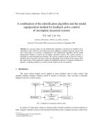
Báo cáo " A combination of the identification algorithm and the modal superposition method for feedback active control of incomplete measured systems " doc
... controlled by the identification algorithm. The numerical simulations are taken when the sensor is placed at the distances L/4, L/2 and L from the base. In Fig 3, the shapes of the 1st mode, the 3rd ... subinterval T k ended, the information known can be used only in the next subinterval T k+1 to calculate u [k+1] (t). Using the delayed information, the control force u c acting on the significant ... and the locations of the sensors. The numerical simulation is applied to a base excited cantilever beam to illustrate the algorithm. The effects of the time delay and the location of sensor...
Ngày tải lên: 28/03/2014, 13:20

Báo cáo " A combination of the identification algorithm and the modal superposition method for feedback active control of incomplete measured systems" doc
... term. The magnitude of the error term depends on the number and the locations of the sensors. The numerical simulation is applied to a base excited cantilever beam to illustrate the algorithm. The ... subinterval T k ended, the information known can be used only in the next subinterval T k+1 to calculate u [k+1] (t). Using the delayed information, the control force u c acting on the significant ... produce the required forces. When only the responses can be measured, the method is called feedback active control. In recent years, the active control method has been widely used to reduce the...
Ngày tải lên: 28/03/2014, 13:20

báo cáo hóa học: " The shrinking projection method for solving generalized equilibrium problems and common fixed points for asymptotically quasij-nonexpansive mappings" potx
... addition, there are several other pro- blems, for example, the complementarity problem, fixed point problem and optimiza- tion problem, which can also be written in the form of an EP( f). In other ... and only if x = y . By the Hahn-Banach theorem, J(x) for each x ẻ E, for more details see [35,36]. Remark 1.1.ItisalsoknownthatifE is uniformly smooth, then J is uniformly norm-to-norm continuous ... scheme based on the shrinking projection method for finding a common element of the set of solutions of the generalized mixed equilibrium problems and the set of common fixed points for a pair of...
Ngày tải lên: 21/06/2014, 02:20