the compositional logic of the covenant code

Nonlinear Model Predictive Control: Theory and Algorithms (repost)
... many of the theoretical and structural properties of NMPC developed in the first part are used when looking at the performance of numerical algorithms The basic theme of the first part of the book ... represents the total mass of arm, rotor and platform and m is the mass of arm, r denotes the distance from the A/R joint to the arm center of mass and I , J and D are the moment of inertia of the arm ... Proof The proof is analogous to the proof of Theorem 2.20 with the obvious modifications 2.4 Stability of Sampled Data Systems We now investigate the special case in which (2.31) represents the...
Ngày tải lên: 11/06/2014, 08:23

Báo cáo hóa học: "Research Article Neural Network Adaptive Control for Discrete-Time Nonlinear Nonnegative Dynamical Systems" ppt
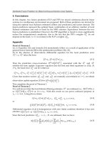
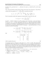
... the proof of Theorem 4.1 below For the remainder of the paper we assume that there exists a gain matrix K ∈ Rm×nx such that A BK is nonnegative and asymptotically stable, where A and B have the ... to each individual compartment For the statement of the next theorem, recall the definitions of W and W k , k ∈ Z , given in Theorem 4.1 Theorem 5.1 Consider the discrete-time nonlinear uncertain ... assumption is made in the proof of Theorem 5.1 B Proof of Theorem 5.1 In this appendix, we prove Theorem 5.1 First, define Wu k where ⎧ ⎨0, if ui k < 0, Wui k i ⎩Wi k , otherwise, block-diag Wu1...
Ngày tải lên: 22/06/2014, 11:20

ON STABILITY ZONES FOR DISCRETE-TIME PERIODIC LINEAR HAMILTONIAN SYSTEMS ˘ VLADIMIR RASVAN Received potx
... the symmetric with respect to the unit circle of the complex plane (in the sense of inversion) of the eigenvalues of −Bk Indeed, if μ is an eigenvalue of −Bk , then det μI + Bk = (1.10) Stability ... [19], the results of Liapunov for the central stability zone of ı (1.1) have been extended to the case when p(t) has values of both signs [22] but the cited reference contained no proofs The proofs ... stability zone is delimited as in the previous case The instability zones are nevertheless more complicated from the point of view of the representation of A(λ) there An instability zone may contain...
Ngày tải lên: 23/06/2014, 00:20

Báo cáo sinh học: " Heritability of longevity in Large White and Landrace sows using continuous time and grouped data models" ppsx
... weaning) Animals were censored either at the date of the last weaning, if they were alive at the time of data collection or at the 9th weaning if they were alive at the 10th farrowing Only sows born ... justified such choices: first, the Laplace approximation of the posterior density of the genetic variance requires the repeated inversion of the Hessian matrix of the log-posterior density, which ... reviewed the text VD further developed the idea, helped with the analysis, wrote parts of the text and helped with the revision of existing parts JP did the statistical analysis and helped to write the...
Ngày tải lên: 14/08/2014, 13:21

Adaptive control and neural network control of nonlinear discrete time systems
... A the set of all real numbers the set of all integers the set of all integers which are not less than integer t the Euclidean norm of vector A or the induced norm of matrix A the transpose of ... vector the determinant of matrix A the set of eigenvalues of A the maximum eigenvalue of real symmetric matrix A the minimum eigenvalue of real symmetric matrix A the absolute value of number a the ... i.e., the absolute values of the gains are unknown while the signs of the control gains are known In the consequent Chapter 4, we will further remove the assumption on control directions The robust...
Ngày tải lên: 14/09/2015, 08:39

Changes of temperature data for energy studies over time and their impact on energy consumption and CO2 emissions. The case of Athens and Thessaloniki – Greece
... the meteorological stations of the National Observatory of Athens (NOA) [8] and of the Aristotle University of Thessaloniki (AUTh) [9] The results for the two decades are compared and the existing ... in the range of to 9% in Thessaloniki, depending on the base temperature, with the highest changes observed at the lowest base temperatures The increase of the yearly values of CDD was in the ... values of HDD were reduced in the second decade, while the monthly and yearly values of CDD were increased The reduction in the yearly values of HDD was in the range of 9.5 to 22% in Athens,...
Ngày tải lên: 05/09/2013, 16:10
Tài liệu ADVANCES IN DISCRETE TIME SYSTEMS docx
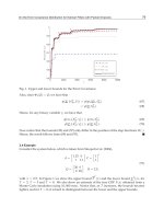
... the condition (23) This completes the proof Based on Lemma 4.1(ii), we have the following theorem The proof is similar to that of Theorem 4.2, and is thus omitted Theorem 4.3 Given γ and K, the ... calculating all these controllers by using Algorithm in this ex‐ ample In order to illustrate further the results, we give the trajectories of state of the system (15) with the state feedback of the form ... 0satisfies the discrete-time Riccati equation (20); then we have the following lemma Lemma 3.2 Suppose that the conditions i-ii of Theorem 3.1 hold, then the both AK ∗ and AK are stable Proof: Suppose...
Ngày tải lên: 14/02/2014, 09:20


Discrete Time Systems Part 1 pdf
... Methods The models of the DF is as general as the models of particle filters, whereas the models of the extended Kalman filter (EKF) are linear functions of the disturbance and observation noises The ... the number, m, of possible values of the approximate initial random vector xd (0) is increased and the initial step of the DF is repeated from the beginning; otherwise, the metrics of admissible ... through the other nodes are pruned Hence, the implementation complexity of the DF does not increase with time The number MN is one of the parameters determining the implementation complexity and the...
Ngày tải lên: 20/06/2014, 01:20

Discrete Time Systems Part 2 potx
... and therefore the estimation error is asymptotically stable This ends the proof of Theorem 2.1 Remark 2.2 The Schur lemma and its application in the proof of Theorem 2.1 are detailed in the Appendix ... α α K1 = λ= 2γ Proof The proof of this theorem is an extension of that of Theorem 2.1 Let us consider the same Lyapunov-Krasovskii functional defined in (8) We show that if the convex optimization ... ⎣ ⎦⎣ ⎦ Further, in parallel with the FLP we offer the other algorithm for fusion prediction 3.2 The prediction of fusion filter (PFF Algorithm) This algorithm consists of two parts The first...
Ngày tải lên: 20/06/2014, 01:20
Discrete Time Systems Part 3 ppt
... (13) is given in Theorem ˆ t+Δ d Unbiased property of the fusion estimate xPFF is proved by using the same method as in Theorem This completes the proof of Theorem Proof of Theorem By integrating ... completes the proof of Theorem Proof of Theorem a., c Equations (18) and (19) immediately follow from the general fusion formula for the filtering problem (Shin et al., 2006) b Derivation of observation ... (56) Thus, the right hand side indicates the amount of the reduction of the estimation error by the fixed-point smoothing over the optimal filtering The fixed-interval smoothing We consider the fixed-interval...
Ngày tải lên: 20/06/2014, 01:20
Discrete Time Systems Part 4 pptx
... shows the time evolution of the mean value (over 500 experiments) of both states and of their estimated values using the classic and the robust predictors It can be verified that the estimates of the ... note that the mean of the noises depend on the uncertain parameters of the model The same applies to the covariance matrix Linear robust estimation 4.1 Describing the model Consider the following ... Clafiore (2001) The advances of technology lead to smaller and more sensible components The degradation of these component became more often and remarkable Also, the number and complexity of these components...
Ngày tải lên: 20/06/2014, 01:20

Discrete Time Systems Part 5 potx
... verify the effectiveness of the stochastic optimal preview tracking design theory In the appendices we present the proof of the proposition, which gives the necessary and sufficient conditions of the ... concludes the proof of sufficiency Necessity: Because of arbitrariness of the reference signal rd(·), by considering the case of rd(·) ≡ 0, one can easily deduce the necessity for the solvability of the ... over the finite horizon [0,N], using the information available on the known part of the reference signal rd(·) and minimizing the sum of the energy of zd(k), for the given initial mode i0 and the...
Ngày tải lên: 20/06/2014, 01:20

Discrete Time Systems Part 6 pptx
... condition for (6) Thus we complete the proof Remark The proof of Theorem is based on the equivalence between and of Finsler’s lemma It also provides an alterative proof of Theorem if we note that (5) ... experience, the choose of different vectors and their sequence affect the result The following simple result is the consequence of the equivalence of and in Finsler’s Lemma Output Feedback Control of ... the comparison of Theorem and Theorem Some phenomenons (the solvability of Theorem and Theorem depends on the l and m When m > l, Theorem tends to have a higher solvability than Theorem And vise...
Ngày tải lên: 20/06/2014, 01:20

Discrete Time Systems Part 7 ppt
... Proof: We follow similar lines of proof of Theorem 3.1 for the stability of the system (23) Then, the result is straightforward 5.2 Robust observer analysis Now, we extend the result for the ... combining the Lyapunov method for proving the discrete time optimal LQR control problem with the above extension of the discrete time bounded real lemma, the argument of completion of squares of Furuta ... + Bd K ) x (k − dk ) (6) In the following section, we consider the robust stability of the closed-loop system (5) and the stability of the closed-loop system (6) The following lemma is useful...
Ngày tải lên: 20/06/2014, 01:20
Discrete Time Systems Part 8 pot
... a way that the j-step prediction is based on the previous step predictions The prediction method Yang et al (2009) is further developed here for the compensation of the effect of the nonlinear ... 1) , the values of parameter estimates at the (k + 1)-th step are same as those at the (k + n − 2)-th step While the estimate values will be updated outside of this region The threshold of the ... small neighborhood of zero To avoid the singularity problem, we may take advantage of the a priori information of the lower bound of gm , i.e g , to revise the update m ˆ law of gm (k) in (38)...
Ngày tải lên: 20/06/2014, 01:20

Discrete Time Systems Part 9 ppt
... for the other agents, they are unaware of either the reference trajectory or the existence of the leader and the outputs of their neighbors are the only external information available for them, ... radius of A, i.e ρ( A) = max{| λ( A)|} and ρ( A) < 1, then we can obtain X ( k + 1) = O [ 1] (5.21) 250 Discrete Time Systems 5.6 Proof of Theorem 5.1 In the following, the proof of mathematic ... the influence of the other agents towards Agent i Hereinafter, xi (t) is the weighted average of states of agents in the neighborhood of Agent i, i.e., ¯ xi (t) = ∑ j ∈N i where the nonnegative...
Ngày tải lên: 20/06/2014, 01:20

Discrete Time Systems Part 10 pdf
... mass-change periods The magnitude of these errors is also related to the rapid changes of the reference vref in the programmed maneuvers In the Fig 5, the time evolution of the actuator thrust ... the forces are compared within the three periods of transients One observes that the intervention of the controller after a sudden change of mass occurred immediately Also the transients of these ... saturation values of the thrusters are achieved Since τ 2n is fixed by the controller, the only countermeasure to be applied lays in the fact that the controller always choose the lower τ 2n of the two...
Ngày tải lên: 20/06/2014, 01:20

Discrete Time Systems Part 11 potx
... steps of those taken in the proof of Theorem are taken The main differences are related to i) the size and structure of the matrices and ii) the manipulations done to keep the convexity of the ... issue of Theorem is the use of one matrix X i for each submode This is possible because of the switched nature of the system that reaches only the vertices of the polytope Example Consider the ... robust stability of the considered system Proof Following the proof given for Theorem 1, it is possible to conclude that the positivity of (14) is assured with the hypothesis of P (α) = P (α)...
Ngày tải lên: 20/06/2014, 01:20
Discrete Time Systems Part 12 ppt
... seen from the proof of Theorem that what we really need is the equation (4.4) Therefore, Theorem can be extended to the case where the subsystem descriptor matrices are different as in the following ... A| ≡ The finite eigenvalues of the matrix pair ( E, A), that is, the solutions of | zE − A| = 0, and the corresponding (generalized) eigenvectors define exponential modes of the system If the finite ... system (1) The stability of the system when the elements of A(⊗) are not known exactly is of major interest The uncertainty can arise from perturbations in the system parameters because of changes...
Ngày tải lên: 20/06/2014, 01:20