partial differential equations in engineering pdf

Báo cáo y học: "Modelling of oedemous limbs and venous ulcers using partial differential equations" pdf

Ngày tải lên : 13/08/2014, 23:20

9
282
0

Partial Differential Equations part 1

Ngày tải lên : 28/10/2013, 22:15

... America). Chapter 19. Partial Differential Equations 19.0 Introduction The numerical treatment of partial differential equations is, by itself, a vast subject. Partial differential equations are at ... Numerical Recipes dealing with partial differential equations alone. (The references [1-4] provide, of course, available alternatives.) In most mathematics books, partial differential equations (PDEs) ... and (19.0.2) both deﬁne initial value or Cauchy problems: If information on u (perhaps including time derivative information) is 827 830 Chapter 19. Partial Differential Equations Sample page from...

8
393
0

Partial Differential Equations part 2

Ngày tải lên : 07/11/2013, 19:15

... various ways of improving the accuracy of ﬁrst-order upwind differencing. In the continuum equation, material originally a distance v∆t away 840 Chapter 19. Partial Differential Equations Sample page ... own domain of dependency determined by the choice of points on one time slice (shown as connected solid dots) whose values are used in determining a new point (shown connected by dashed lines). ... viscosity to the equations, modeling the way Nature uses real viscosity to smooth discontinuities. A good starting point for trying out this method is the differencing scheme in §12.11 of [1] ....

14
433
0

Tài liệu Partial Differential Equations part 3 pptx

Ngày tải lên : 15/12/2013, 04:15

... accurate in time for the scales that we are interested in. The second answer is to let small-scale features maintain their initial amplitudes, so that the evolution of the larger-scale features of interest ... form again and in practice usually retains the stability advantages of fully implicit differencing. Schr ¨ odinger Equation Sometimes the physical problem being solved imposes constraints on ... steps of the other kind, to drive the small-scale stuff into equilibrium. Let us now see where these distinct differencing schemes come from: Consider the following differencing of (19.2.3), u n+1 j −...

7
354
0

Tài liệu Partial Differential Equations part 4 ppt

Ngày tải lên : 15/12/2013, 04:15

... underlying PDEs, perhaps allowing second-order spatial differencing for ﬁrst-order -in- space PDEs. When you increase the order of a differencing method to greater than the order of the original ... 100 mesh points requires at least 100 times as much computing. You generally have to be content with very modest spatial resolution in multidimensional problems. Indulge us in offering a bit of ... U m (u n+(m−1)/m , ∆t) (19.3.20) 854 Chapter 19. Partial Differential Equations Sample page from NUMERICAL RECIPES IN C: THE ART OF SCIENTIFIC COMPUTING (ISBN 0-521-43108-5) Copyright (C) 1988-1992...

5
374
0

Tài liệu Partial Differential Equations part 5 ppt

Ngày tải lên : 15/12/2013, 04:15

... equations u j−1 + T · u j + u j+1 = g j ∆ 2 (19.4.29) Here the index j comes from differencing in the x-direction, while the y-differencing (denoted by the index l previously) has been left in ... the number of equations by a factor of two. Since the resulting equations are of the same form as the original equation, we can repeat the process. Taking the number of mesh points to be a power ... get the y-values on these x-lines. Then ﬁll in the intermediate x-lines as in the original CR algorithm. The trick is to choose the number of levels of CR so as to minimize the total number of...

7
379
0

Tài liệu Partial Differential Equations part 6 doc

Ngày tải lên : 15/12/2013, 04:15

... become available. In other words, the averaging is done in place” instead of being “copied” from an earlier timestep to a later one. If we are proceeding along the rows, incrementing j for fixed ... mentioned in §19.0, relaxation methods involve splitting the sparse matrix that arises from finite differencing and then iterating until a solution is found. There is another way of thinking about ... get the y-values on these x-lines. Then fill in the intermediate x-lines as in the original CR algorithm. The trick is to choose the number of levels of CR so as to minimize the total number of...

9
329
0

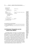
Tài liệu Integration of Ordinary Differential Equations part 5 pdf

Ngày tải lên : 24/12/2013, 12:16

... are not particularly good for differential equations that have singular points inside the interval of integration. A regular solution must tiptoe very carefully across such points. Runge-Kuttawithadaptivestepsize ... encountered in practice, is discussed in §16.7.) 726 Chapter 16. Integration of Ordinary Differential Equations Sample page from NUMERICAL RECIPES IN C: THE ART OF SCIENTIFIC COMPUTING (ISBN 0-521-43108-5) Copyright ... remind you once again that scaling of the variables is often crucial for successful integration of differential equations. The scaling “trick” suggested in the discussion following equation (16.2.8)...

9
486
0

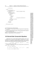
Tài liệu Integration of Ordinary Differential Equations part 6 pdf

Ngày tải lên : 24/12/2013, 12:16

... for this is explained below). This is so even 732 Chapter 16. Integration of Ordinary Differential Equations Sample page from NUMERICAL RECIPES IN C: THE ART OF SCIENTIFIC COMPUTING (ISBN 0-521-43108-5) Copyright ... FURTHER READING: Stoer, J., and Bulirsch, R. 1980, Introduction to Numerical Analysis (New York: Springer-Verlag), § 7.2.14. [1] Gear, C.W. 1971, Numerical Initial Value Problems in Ordinary Differential ... is a particular class of equations that occurs quite frequently in practice where you can gain about a factor of two in efﬁciency by differencing the equations directly. The equations are second-order...

3
395
0

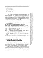
Tài liệu Integration of Ordinary Differential Equations part 8 pdf

Ngày tải lên : 24/12/2013, 12:16

... surprise in store when you first have to fix a problem in a predictor-corrector routine. Let us first consider the multistep approach. Think about how integrating an ODE is different from findingthe integral ... effect. Therefore, the integration steps of a predictor-corrector method are overlapping, each one involving several stepsize intervals h, but extending just one such interval farther than the previous ... applications. We are willing, however, to be corrected. CITED REFERENCES AND FURTHER READING: Gear, C.W. 1971, Numerical Initial Value Problems in Ordinary Differential Equations (Englewood Cliffs,...

6
457
0

Tài liệu Partial Differential Equations part 7 doc

Ngày tải lên : 24/12/2013, 12:16

... a whole line along that dimension simultaneously. Line relaxation for nearest-neighbor coupling involves solving a tridiagonal system, and so is still efﬁcient. Relaxing odd and even lines on ... com- puted.#define NGMAX 15 void mglin(double **u, int n, int ncycle) Full Multigrid Algorithm for solution of linear elliptic equation, here the model problem (19.0.6). On input u[1 n][1 n] contains the ... double **res, int nf); void copy(double **aout, double **ain, int n); void fill0(double **u, int n); void interp(double **uf, double **uc, int nf); void relax(double **u, double **rhs, int n); void...

18
349
0

Functional analysis sobolev spaces and partial differential equations

Ngày tải lên : 04/02/2014, 11:10

... occur in a wide range of questions, in both pure and applied mathematics. They appear in linear and nonlinear PDEs that arise, for example, in differential geometry, harmonic analysis, engineering, ... Recall that in general, a pointwise limit of continuous maps need not be continuous. The linearity assumption plays an essential role in Theorem 2.2. Note, however, that in the setting of Theorem ... not achieved (see, e.g., Exercise 1.17). The theory of min- imal surfaces provides an interesting setting in which the primal problem (i.e., inf x∈E {ϕ(x) + ψ(x)}) need not have a solution, while...

614
1.9K
1

Tài liệu AN INTRODUCTION TO PARTIAL DIFFERENTIAL EQUATIONS ppt

Ngày tải lên : 16/02/2014, 15:20

... comments at pincho@techunix.technion.ac.il. We will maintain a webpage with a list of errata at http://www.math.technion.ac .il/∼pincho/PDE .pdf. AN INTRODUCTION TO PARTIAL DIFFERENTIAL EQUATIONS A ... fourth-order equation. r Linear equations Another classiﬁcation is into two groups: linear versus nonlinear equations. An equation is called linear if in (1.1), F is a linear function of the unknown ... frequently in all areas of physics and engineering. Moreover, in recent years we have seen a dramatic increase in the use of PDEs in areas such as biology, chemistry, computer sciences (particularly in relation...

385
508
2

Tài liệu Boundary Value Problems, Sixth Edition: and Partial Differential Equations pptx

Ngày tải lên : 17/02/2014, 14:20

... other kinds of linear, homogeneous equations. Later, we will be using the same principle on partial differential equations. To be able to satisfy an unrestricted initial condition, we need two linearly ... Ordinary Differential Equations multiple of π ,sincesin(π ) = 0, sin(2π) = 0, etc., and integer multiples of π are the only arguments for which the sine function is 0. The equation λa =π , in ... exercises are in ix Contents Preface ix CHAPTER 0 Ordinary Differential Equations 1 0.1 Homogeneous Linear Equations 1 0.2 Nonhomogeneous Linear Equations 14 0.3 Boundary Value Problems 26 0.4 Singular...

515
1K
0

Partial Differential Equations and Fluid Mechanics doc

Ngày tải lên : 14/03/2014, 10:20

... describing the body as inhomogeneous we are referring to the fact that the averaged body has properties that change from one material point to another. It is important to keep this distinction in mind. ... mathematical properties of unsteady three- dimensional internal flows of chemically reacting incompressible shear- thinning (or shear-thickening) fluids. Assuming that we have Navier’s slip at the impermeable ... primarily interested in the fluid that is carried along and reacting with our fluid of interest having associated with it a much smaller and in fact ignorable density. Thus, as mentioned earlier, in the...

271
580
0

Entropy and partial differential equations evans l c

Ngày tải lên : 17/03/2014, 14:29

... heating” and  m k=1 P k dX k as in nitesimal working” for a process. In this chapter however there is no notion whatsoever of anything changing in time: everything is in equilibrium. Terminology. ... entropy. Proof. 1. Fix a point (T ∗ ,V ∗ ) in Σ and consider a Carnot heat engine as drawn (assuming Λ V > 0): 36 (iii) the use of entropy in providing variational principles. Another ongoing issue will ... system in equilibrium, and so could immediately discuss energy, entropy, temperature, etc. This point of view is static in time. In this chapter we introduce various sorts of processes, involving...