matrix factorizations and direct solution of linear systems

Stability analysis and controller design of linear systems with random parametric uncertaintie
... transformation matrix of the augmented system Ai matrix of gPC expansion coefficients of A(∆) associated with the i-th orthogonal polynomial ¯ Aij the ij-th n-by-n submatrix of A mp the p-th moment of x ... investigate the influences of both the structure of the original system and the random uncertain parameters on the stability and performance of the system, and demonstrate the application of this finding ... the control of the probability distribution of the system states The main contribution of this thesis is the application of the gPC theory to the analysis and control of systems with random parametric...
Ngày tải lên: 10/09/2015, 09:25

Analysis and Control of Linear Systems - Chapter 0 pptx
... Cataloging-in-Publication Data [Analyse des systèmes linéaires/Commande des systèmes linéaires eng] Analysis and control of linear systems analysis and control of linear systems/ edited by Philippe de Larminat p cm ... equations of measurement for continuous systems 2.1.3 Case of linear systems 2.1.4 Case of continuous and invariant linear systems ... Calculation method of the transition matrix e A(t -t0 ) 2.2.5 Application to the modeling of linear discrete systems 2.3 Scalar representation of linear and invariant systems ...
Ngày tải lên: 09/08/2014, 06:23

Analysis and Control of Linear Systems - Chapter 1 pptx
... at 5%) and ω t m according to the damping ξ Figure 1.21 ω0 tr and ω0 tm according to the damping ξ 30 Analysis and Control of Linear Systems The alternation of slow and fast variations of product ... final value of the response at the end of time T, which is called time constant of the system The response reaches 0.63 K in T and 0.95 K in T 24 Analysis and Control of Linear Systems Figure ... jf0 20 Analysis and Control of Linear Systems Table 1.1 sums up the features of a system’s transfer function, the existence conditions of its frequency response and the possibility of performing...
Ngày tải lên: 09/08/2014, 06:23

Analysis and Control of Linear Systems - Chapter 3 pps
... Analysis and Control of Linear Systems 3.2.2 Delay and lead operators The concept of an operator is interesting because it enables a compact formulation of the description of signals and systems ... development of X (z) by polynomial division according to 86 Analysis and Control of Linear Systems the decreasing powers of z −1 or apply the method of deviations, starting from the definition of the ... ) and y f (k ) designate respectively the free response and the forced response of the system Unlike the continuous case, the solution involves a sum, and not an integration, of powers of A and...
Ngày tải lên: 09/08/2014, 06:23
Analysis and Control of Linear Systems - Chapter 4 ppt
... 110 Analysis and Control of Linear Systems The object of this chapter is to describe certain structural properties of linear systems that condition the resolution of numerous control problems ... and W t a basis of the canceller at the left of W (i.e a maximal solution of equation WtW = {0}), a basis of LV is obtained by directly preserving only the independent columns of LV A basis of ... illustrated with respect to the existence of solutions, the existence of stabilizing solutions and flexibilities offered in terms of poles positions (concept of fixed poles) This is illustrated in...
Ngày tải lên: 09/08/2014, 06:23
Analysis and Control of Linear Systems - Chapter 5 pptx
... proximity of ν0 152 Analysis and Control of Linear Systems Figure 5.1 Typical power spectrum of an MA (left) or AR (right) model In the case of a single denominator (nc = 0), we talk of an AR ... filter, in the sense of the second momentum of the prediction error y[k] − y [k], among all linear filters without direct transmission on y[k] ˆ 156 Analysis and Control of Linear Systems This prediction ... my )) ∀κ ∈ Z [5.18] 146 Analysis and Control of Linear Systems are independent of index k, i.e independent of the time origin σy = ryy [0] is the r [κ] variance of the signal considered yy2 is...
Ngày tải lên: 09/08/2014, 06:23
Analysis and Control of Linear Systems - Chapter 6 ppsx
... Analysis and Control of Linear Systems u (t ) = − K x(t ) + e(t ) [6.2] where K is an m × n matrix (Figure 6.1) and signal e(t ) represents the input of the looped system The equations of the looped ... ( H , F ) is detectable [6.41] 174 Analysis and Control of Linear Systems there is a unique matrix P , symmetric and positive semi-defined, solution of the following equation (called discrete ... control, whereas the increase of ξ leads to better dynamics 164 Analysis and Control of Linear Systems Figure 6.2 Stabilization by pole placement 6.3 Reconstruction of state and observers 6.3.1 General...
Ngày tải lên: 09/08/2014, 06:23
Analysis and Control of Linear Systems - Chapter 7 docx
... 196 Analysis and Control of Linear Systems in performing the roles of the procedure, in connection with a structure and behavior of components They are used for the design of procedure monitoring, ... one hand, the problem of identification (and also the problem of simulation and control) is made much easier by the computing tool and is already well known in data analysis (linear or non -linear ... Analysis and Control of Linear Systems recording of a specific response We need to be aware of the fact that it is essential to have a little, even very little, noise on the responses and, irrespective...
Ngày tải lên: 09/08/2014, 06:23

Analysis and Control of Linear Systems - Chapter 8 ppsx
... Analysis and Control of Linear Systems directly apply the results of the previous section From a theoretical point of view, we can, however, return by transforming [8.13] into a system directly ... λM and λm are respectively the poles with the highest and smallest negative real part, of absolute value N OTE 8.4 For standard linear systems [8.1], the poles are directly the eigenvalues of ... in the direct chain of control One solution can be to increase the length of words intervening in the calculations of the integral action A second solution consists of storing the part of ekT...
Ngày tải lên: 09/08/2014, 06:23
Analysis and Control of Linear Systems - Chapter 9 pot
... SIGUERDIDJANE and Martial DEMERLÉ 254 Analysis and Control of Linear Systems Figure 9.2 General block diagram The open loop transfer function of this chain is the product of transfer functions of all ... equation of n order The roots of this equation are of strictly negative real part if and only if the terms of this first column of the table have the same sign and are not zero Statement of Routh’s ... in CL and (b) frequency response in CL 258 Analysis and Control of Linear Systems When the system has good damping, let ξ be the value of the damping coefficient delimited between 0.4 and 0.7,...
Ngày tải lên: 09/08/2014, 06:23
Analysis and Control of Linear Systems - Chapter 10 doc
... Points A and B are thus the separations of cases and Synthesis of Closed Loop Control Systems Between A and B: µ1 µ µ β > and B: µ1 µ µ β < µ1 µ β C µ1 µ β C 317 , i.e µ C > (1st case) and outside ... Analysis and Control of Linear Systems Figure 10.12 Bode graph with insufficient phase margin Figure 10.13 Bode graph in OL of the corrected system Synthesis of Closed Loop Control Systems 297 ... response time and limited precision) On the other hand, irrespective of the linearity of the system, it is not always interesting to have a too extended bandwidth, due to the amplification of noises...
Ngày tải lên: 09/08/2014, 06:23

Analysis and Control of Linear Systems - Chapter 11 pptx
... degree of polynomial A We will assume that the concepts of polynomials division are known, as well as those of PGCD and PPCM of polynomials If G and L are respectively the PGCD and the PPCM of A and ... and R and thus5: number of unknown factors = ∂S + ∂R + A polynomial of degree n has n + coefficients [11.36a] 338 Analysis and Control of Linear Systems The number of equations is the number of ... degree of S and thus that of Bm’, which itself is solution of [11.30(d)] For this equation, there is no constraint on being proper and we will set the uniqueness of the solution by retaining that of...
Ngày tải lên: 09/08/2014, 06:23

Analysis and Control of Linear Systems - Chapter 12 pptx
... ideas of the method, starting with the form of the model, the quadratic criterion and up to the examination of adjustment parameters The formalism and the 390 Analysis and Control of Linear Systems ... , H j , J j are single solutions of Diophantus equations, which are obtained by equality of the inputs and output of transfer functions of equations [12.1] and [12.3] and they are solved recursively: ... the number of estimated values of the sequence 376 Analysis and Control of Linear Systems 12.2 Generalized predictive control (GPC) 12.2.1 Formulation of the control law The objective of this section...
Ngày tải lên: 09/08/2014, 06:23

Analysis and Control of Linear Systems - Chapter 13 pptx
... principle than on the concept of state In [CHE 93] we used to talk of direct methods versus iterative methods For linear stationary systems 402 Analysis and Control of Linear Systems In fact, the biggest ... formulated in the standard form of Figure 13.1 408 Analysis and Control of Linear Systems Figure 13.1 Standard feedback diagram The quadripole G , also called a standard model, and feedback K are ... observable part by y is solution of Let us give the idea of the equivalence proof of properties and 2., the equivalence of properties and resulting by duality Methodology of the State Approach...
Ngày tải lên: 09/08/2014, 06:23

Analysis and Control of Linear Systems - Chapter 14 pdf
... 14.5 Area of the complex plane corresponding to the desired performances and to the constraints on the bandwidth 460 Analysis and Control of Linear Systems 14.4.2 Choice of eigenvectors of the closed ... always distinct [14.3] 448 Analysis and Control of Linear Systems The left eigenvectors of matrix A + BK(I − DK)−1 C are noted: u , , un and the output directions: t1 , , tn where (by definition): ... Shift of a set of poles with minimum dispersion 464 Analysis and Control of Linear Systems EXAMPLE 14.4 To illustrate these points, let us take a set of models pertaining to the lateral side of...
Ngày tải lên: 09/08/2014, 06:23

Analysis and Control of Linear Systems - Chapter 15 pot
... the looping of an invariant system of transfer matrix K (s ) and of a response of matrix Θ(t ) (Figure 15.15) Robust H∞/LMI Control 513 Figure 15.15 Structures of the system and of the corrector ... Analysis and Control of Linear Systems where N R and N S form a base of cores of ( Bu T Deu T ) and (C y Dyw ) respectively Inequalities [15.70], calculated on inequalities [15.20.a, b, c] of the ... [15.48] 500 Analysis and Control of Linear Systems a) Robustness of stability b) Robustness of performance Figure 15.10 Upper bounds of the structured single value 15.2.4 Evaluation of structured single...
Ngày tải lên: 09/08/2014, 06:23

Analysis and Control of Linear Systems - Chapter 16 ppt
... λ + t and H (λ ) = λ−1 so ∑ y(t ) = u(t ) 1 530 Analysis and Control of linear Systems 16.4.2 Parallel systems Let ∑1 and ∑ be two systems of transfer functions H1 (λ) = Q1 (λ )−1 P (λ) and H ... algorithm: – solution of the Diophantine equation; ~ ~ – search of RLCM M (λ) of Q(λ), P(λ) ; ~ ~ – P(λ ) and Q(λ ) are quotient polynomials of M (λ ) by Q(λ) and P(λ) respectively The resolution of the ... t Linear Time-Variant Systems 531 16.5 Applications In this section, two types of usage of this algebra are presented in the field of modeling and control 16.5.1 Modeling One of the methods of...
Ngày tải lên: 09/08/2014, 06:23
Robust FiniteTime Stabilization of Linear Systems with Multiple Delays in State and Control
... stabilization of linear singular time delay systems with control delay To the best of our knowledge, finite-time stabilization problem for linear control systems with multiple state and control ... t−mj −hi j=1 t−mj Using the same method of the proof of Theorem 3.1, taking the derivative of V (t) in t along the solution of the closed-loop system and applying the following derived estimations ... nonlinear systems Automatica, 48(2012), 499-504 [5] F Amato, R Ambrosino, C Cosentino, G.De Tommasi, Finite-time stabilization of impulsive dynamical linear systems Nonlinear Analysis: Hybrid Systems, ...
Ngày tải lên: 12/10/2015, 10:29

Finitetime stability and H control of linear discretetime delay systems with normbounded disturbances
... denotes the space of all matrices of (n × r)−dimensions; A⊤ denotes the transpose of matrix A; A is symmetric if A = A⊤ ; I denotes the identity matrix of appropriate dimension Matrix A is called ... control of discrete-time linear systems: Analysis and design conditions, Automatica, 46(2010), 919-924 [3] Zuo Z., Li H., Wang Y., New criterion for finite-time stability of linear discrete-time systems ... control of linear discretetime systems with an interval-like time-varying delay, International Journal of Systems Science, 39(2008), 427-436 [7] Meng Q., Shen Y., Finite-time H∞ control for linear...
Ngày tải lên: 14/10/2015, 08:06
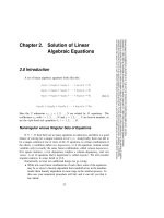
Tài liệu Solution of Linear Algebraic Equations part 1 docx
... Tasks of Computational Linear Algebra • Solution of the matrix equation A·x = b for an unknown vector x, where A is a square matrix of coefficients, raised dot denotes matrix multiplication, and ... “fast matrix inversion” (§2.11) 36 Chapter Solution of Linear Algebraic Equations Coleman, T.F., and Van Loan, C 1988, Handbook for Matrix Computations (Philadelphia: S.I.A.M.) Forsythe, G.E., and ... Moler, C.B 1967, Computer Solution of Linear Algebraic Systems (Englewood Cliffs, NJ: Prentice-Hall) Wilkinson, J.H., and Reinsch, C 1971, Linear Algebra, vol II of Handbook for Automatic Computation...
Ngày tải lên: 15/12/2013, 04:15