homicide injury miscarriage and talion exodus 21 12 14 18 27

... 8.10 Notes and Extensions 8.11 Problems References 211 211 214 217 222 225 227 232 237 241 246 ... Moore and YangQuan Chen Distributed Consensus in Multi-vehicle Cooperative Control Wei Ren and Randal W Beard Control of Singular Systems with Random Abrupt Changes El-Kébir Boukas Positive 1D and ... Nonlinear and Adaptive Control with Applications Alessandro Astolfi, Dimitrios Karagiannis and Romeo Ortega Identification and Control Using Volterra Models Francis J Doyle III, Ronald K Pearson and...

Ngày tải lên: 11/06/2014, 08:23

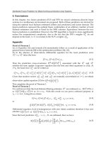
... spectrum of A, let C1 {s ∈ C : |s| ≥ 1}, n×n and let A ∈ R in 2.4 be partitioned as A A11 A12 , A21 A22 2.6 where A11 ∈ Rm×m , A12 ∈ Rm× n−m , A21 ∈ R n−m ×m , and A22 ∈ R n−m × n−m are nonnegative ... 11 I W Sandberg, “On the mathematical foundations of compartmental analysis in biology, medicine, and ecology,” IEEE Transactions on Circuits and Systems, vol 25, no 5, pp 273 279 , 1978 12 H Maeda, ... Chellaboina, and E August, “Stability and dissipativity theory for discrete-time non-negative and compartmental dynamical systems,” International Journal of Control, vol 76, no 18, pp 184 5 186 1, 2003...

Ngày tải lên: 22/06/2014, 11:20

... periodic and skew-periodic boundary value problems and, further, the discrete-time parametric resonance 12 Stability zones for discrete Hamiltonian systems References [1] C D Ahlbrandt and A C ... associated boundary value problems A good reference is the book of Ahlbrandt and Peterson [1], the papers of Erbe and Yan [7–10] and the long list of papers by Bohner et al among which we cite the ... systems Besides the already cited reference of Halanay and R˘ svan [14] , we mention here [23, 24] a where the line of Kre˘n [19, 18] is followed and attempts are made to adapt those techı niques borrowed...

Ngày tải lên: 23/06/2014, 00:20

... 0.08 and 0 .14 (s.e 0. 012 - 0.026) for the continuous time and between 0.08 and 0.13 (s.e 0. 012 0.025) for the grouped data models Whatever the breed, heritabilities are highest for the sire and ... 0 .140 (0.024) 0.077 (0. 012) 0 .140 (0.025) 0.077 (0. 012) Sire mgs dam 0.169 a (0. 018) 0.097 (0.023) 0.166 b (0.017) 0.095 (0.023) Sire dam 0.202 (0.035) 0.113 (0. 018) 0.197 (0.034) 0.111 (0. 018) ... sire-maternal grandsire, sire-dam, sirematernal grandsire-dam within maternal grandsire and animal models with Weibull and grouped data models in both breeds They ranged from 0.08 to 0 .14 (s.e 0. 0120 .026)...

Ngày tải lên: 14/08/2014, 13:21

... function based adaptive NN control has been widely studied in both discrete-time [145 ,146 ] and continuous-time [125 ,147 ,148 ] Based on implicit function theory, adaptive NN control using backstepping ... signal and NN weights norm 139 6.7 Discrete Nussbaum gain N (x(k)) and its argument x(k) 140 6.8 Reference signal and system output 140 ix ... signal and NN weights norm 141 6.10 Discrete Nussbaum gain 141 6.11 NN learning error 142 7.1 System output and...

Ngày tải lên: 14/09/2015, 08:39

... Temperature 18 16 14 12 10 18 16 14 12 10 18 16 14 12 10 18 16 14 12 10 18 16 14 12 10 18 16 14 12 10 18 16 14 12 10 18 16 14 12 10 1983 – 1992 47 22 131 84 46 21 244 184 128 80 44 266 204 146 95 ... Total Base Temperature 18 16 14 12 10 18 16 14 12 10 18 16 14 12 10 18 16 14 12 10 18 16 14 12 10 18 16 14 12 10 18 16 14 12 10 18 16 14 12 10 1983 – 1992 90 53 28 12 215 159 108 67 37 354 292 ... 11.97 15.74 21. 34 26.34 28.79 28.30 24.16 19.43 14. 64 11 .18 18.50 1983-2002 9.58 9.90 11.72 15.75 20.63 25.38 27. 96 27. 53 23.83 18. 87 14. 26 10.65 18. 00 1983-1992 6.13 6.86 9.83 14. 58 18. 86 23.31...

Ngày tải lên: 05/09/2013, 16:10

... } J E = limE x T (k)Qx(k) + u T (k)Ru(k) k→∞ 11 12 Advances in Discrete Time Systems T Define Q = C1T C1 and R = D12 D12 and suppose thatC1T D12 = 0, then J E may be rewritten as { } J E = limE ... combined LQG/H ∞ control problem in the T special case of Q = C1T C1 and R = D12 D12 and C1T D12 = arisen from Bernstein & Haddad (1989) and Haddad et al (1991) is a mixed H 2/H ∞ control problem Based ... X8>0 0.3578 − 0.3167 − 2.1049 p1,2 = − 0.0584 ± j0.5939 X9>0 0 .216 6 − 0.3360 − 2. 121 2 p1,2 = − 0.0680 ± j0.6 427 10 X 10 > − 0.2 927 Table The calculating results of algorithm 3.1 To determine...

Ngày tải lên: 14/02/2014, 09:20

Ngày tải lên: 06/03/2014, 17:20

... 0 .216 0.242 0.191 0.0 0.166 -0 .184 0 .145 -0.332 0 .129 -0.453 0. 114 1.377 0.169 0.768 0.175 0.424 0.162 0 .184 0 .145 0.130 -0 .148 0. 118 1.499 0.134 0.908 0 .145 0.569 0.139 0.332 0 .129 0 .148 0. 118 ... -0.355 0 .277 -0.592 0 .216 -0.768 0.175 -0.908 0 .145 -1.023 0 .124 -1 .120 0.106 -1.199 0.093 1.005 0.315 0.355 0 .277 0.0 0.230 -0.242 0.191 -0.424 0.162 -0.569 0.139 -0.690 0. 121 -0.789 0.106 1 . 218 0.223 ... 1.023 0 .124 0.690 0. 121 0.453 0. 114 1.690 0.092 1 .120 0.106 0.789 0.106 1.764 0.079 1.199 1. 818 0.093 0.069 Table Approximate Discrete Random Variables the best Approximating the Gaussian Random...

Ngày tải lên: 20/06/2014, 01:20

... (36) and (37) with aij = and ad = for all i, l = 1, , q, j = 1, , s and m = 1, , r, where lm d s = max (si ) and r = max (ri ) Indeed, if there exist subsets S1 , S1 ⊂ {1, , q }, S2 ⊂ {1, , s} and ... Phase plot of the system d d a11 = 1, b11 = 1, a21 = −1, b21 = According to the remark 4.1, we must solve the LMI (48) with ⎤ ⎡ 0 d d ˜d ˜ b21 = b21 − a21 = 2, Ad = ⎣0 0 ⎦ 0 −T σ Hence, we obtain ... j = 1,… ,N − 1; (18) The local covariance Pt(ii) and cross-covariance Pt(ij) in (18) are determined by equations (9) and k k (13), respectively; ˆt The initial conditions xFF and PtFF in (17)...

Ngày tải lên: 20/06/2014, 01:20

... Conference, pp 2273 - 2274 , Maryland Chang, K C.; Saha, R K & Bar-Shalom, Y (1997) On Optimal track-to-track fusion, IEEE Transactions on Aerospace and Electronic Systems, Vol 33, No 4, pp 127 1 127 5 52 ... (A.8) k Next using (12) and (18) we will derive equations for the new weights (A.8) Multiplying the first (N-1) homogeneous equations (18) on the left hand side and right hand side by the nonsingular ... =Φ(t+Δ,t k ) (A .12) As we can see from (A.10) and (A .12) if the equality (ijN) δPt(ijN)Φ ( t+Δ,t k ) =Φ ( t+Δ,t k ) δPt+Δ T -1 k (A.13) will be hold then the new weights A(i) ,Δ and B(i) ,Δ satisfy...

Ngày tải lên: 20/06/2014, 01:20

... P11,k|k−1 Mk P11,k|k−1 , (59) P12c,k := P12,k|k−1 + P11,k|k−1 Mk P12,k|k−1 , (60) T P22c,k := P22,k|k−1 + P12,k|k−1 Mk P12,k|k−1 , (61) S1,k := P11c,k − P12c,k , (62) S2,k := P12c,k − P22c,k , (63) S3,k ... where Wk , Vk and X0 denotes the noises and initial state covariance matrices and Sk stands for the cross covariance matrix of the noises Therefore using the properties (8) and (9) and the noises ... the pseudo-inverse does exist Replacing (70) and (69) in (52) and (53), we obtain T P12,k+1|k = P12,k+1|k = P22,k+1|k = −1 T T T = Ak P12c,k P22c,k P12c,k Ak + Ak Sk Ck + Ψ1,k T Ck Sk Ck + Ψ2,k...

Ngày tải lên: 20/06/2014, 01:20

... the system (1) and the performance index (2) Suppose A1, A2 and A3 Then the Stochastic Optimal Fixed-Preview Tracking Problem by State Feedback for (1) and (2) is solvable if and only if there ... Consider the system (1) and the performance index (2) Suppose A1, A2 and A3 Then each of the stochastic optimal tracking problems for (1) and (2) is solvable by state feedback if and only if there ... Markovian Jump Systems 125 to get rid of the mixed terms of rd and x, or θm( k ) and x J d , k ,m( k ) (rd) means the tracking error including the preview information vector θ and can be expressed...

Ngày tải lên: 20/06/2014, 01:20

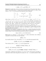
... − P12 P111 P12 ≥ ε P12 +ε For the third situation, noting that we have (21) implies T P12 PT − P111 P12 ≥ ε 12 + ε P12 − ε2 P11 0 ( 1) T T − P12 P111 P12 ≥ εP12 ( 1) ( 1) + εP12 − ε2 P11 (21) ... P11 P12 T T , P12 P2 − ε2 P11 + εP12 + εP12 146 Discrete Time Systems ⎡ Λ2 = ⎣ ⎤ P11 T P12 P2 + ε Λ3 = P11 P12 P12 P ⎦, T + ε[ P12 0] − ε2 11 I ( 1) T T P12 P2 + εP12 P12 ( 1) ( 1) + εP12 − ... − P12 P111 P12 P11 −1 T P [P P ] = P12 11 11 12 For the first situation m = n − m, consider the following inequality: − ( P12 − εP11 ) T P111 ( P12 − εP11 ) ≥ T − T P12 P111 P12 ≥ εP12 + εP12...

Ngày tải lên: 20/06/2014, 01:20

... results in (3), (12) , (14) , (18) considered discrete-time systems with time-invariant delays Gao and Chen (4), Hara and Yoneyama (5), (6) gave robust stability conditions Fridman and Shaked (1) ... Haddad, and Corrado J R (2000) Robust resilient dynamic controllers for systems with parametric uncertainty and controller gain variations, INT J Control, 73(15), pp 140 5- 142 3 P A Iglesias, and ... Control., 43(9), pp 126 5 -126 7 M A Rotea, and Khargonekar P P (1991) H -optimal control with an H ∞ -constraint: the state-feedback case Automatica, 27( 2), pp 307-316 H Rotstein, and Sznaier M (1998)...

Ngày tải lên: 20/06/2014, 01:20

... 81(1): 21 42 URL: http://dx.doi.org/10.1080/0020717070 121 8 333 Ma, H B., Lum, K Y & Ge, S S (2007) Adaptive control for a discrete-time first-order nonlinear system with both parametric and non-parametric ... , n and j = 1, 2, , m Combining (12) and (13), we obtain y(k + n ) = n m i =1 j =1 ∑ θiT Δφi (k + n − i ) + ∑ gj Δu(k − m + j) + y(lk + n) + Δν(k − τ ) (16) Step 1: ˆ ˆ Denote θi (k) and g ... Predictive Control with Asymptotic Output Tracking 215 ˆ ¯ ¯ ˆ ¯ ¯ Define θ (k) and g(k) as estimate of θ and g at the kth step, respectively, and then, the controller will be designed such that...

Ngày tải lên: 20/06/2014, 01:20

... array product The matrices Ci , Dl , Dqi , B1 and B2 are constant and supposed unknown, while Cvi , g1 and g2 are state-dependent and computable arrays and vi is an element of v The generalized propulsion ... ˜ ˜ ˜ Y(k) = [ y1 (k), y2 (k), , yn (k)] T (5 .14) 5.5 Notations and lemmas Define H = [1, 0, , 0] ∈ R T N (5.15) (5.16) From (5.2) and (5 .14) , we have ¯ ¯ [0, x2 (k), , xn (k)] = ΛG A ... of b j1 and b j1 , since b j1 (t) = max(b j1 (t), b j1 ) and b j1 ≥ b j1 , obviously we have ˜2 ˜ b2 (k) ≤ b j1 (k) (5.22) j1 Consider a Lyapunov candidate ˜ Vj (k) = θ j (k) (5.23) and we are...

Ngày tải lên: 20/06/2014, 01:20

... local error Assuming bounded noise vectors δvi and δηi , we can expand (18) and (19) in series of Taylor about the values of undisturbed measures v[tn ] and η[tn ] So it is accomplished T T ∂p ∂pδ ... values of Mb and Ma at the start point O, and MbΔ− , MbΔ+ ,MaΔ+ and MaΔ− are positive and negative variations at instants t A and t B on the points A and B of Fig Here δ(t − ti ) represents the ... −1 ∑ i = l = k − dki and N V3 ( x k ) = ∑ xT Qi xl l − di + k −1 ∑ ∑ i = l =− di + m = k + l − xT Ri xm , m where Qi > and Ri > , and E and P are, respectively, singular and nonsingular matrices...

Ngày tải lên: 20/06/2014, 01:20

... dk = d = 15, where ⎤ ⎡ 0.97 421 0.15116 0.19667 −0.05870 0.0 7144 ⎢ −0. 0145 5 0.88 914 0.26953 0. 1186 6 −0.22047 ⎥ ⎥ ⎢ A = A0 = ⎢ 0.06376 0 .120 56 1.00049 −0.03491 −0. 0276 6 ⎥ (57) ⎥ ⎢ ⎣ −0.05084 0.09254 ... of Theorem lead to K1 = −0. 6129 0.3269 −1.2873 −1.1935 (79) K2 = −0 .219 9 0.1107 −0.6450 −0.4890 (80) Kd1 = −0 .129 1 0.0677 −0.3228 −0.2685 (81) Kd2 = −0.0 518 0. 0271 −0 .129 1 −0.1076 (82) These gains ... −0.1 1185 0.09978 0.04652 0.25867 ⎢ −0.51 718 0.73519 0.57 518 0.40668 −0 .124 72 ⎥ ⎥ ⎢ B = B0 = ⎢ 0.29469 0.31528 1.16420 −0.29922 0.23883 ⎥ , ⎥ ⎢ ⎣ −0.20191 0.19739 0.41686 0.66551 0.11366 ⎦ −0. 1183 5...

Ngày tải lên: 20/06/2014, 01:20

... -0 .12 ≤ 21 ≤ 0 .12, 0 .12 ≤ ⊗22 ≤ 0.24 and b 0 .12 ≤ ⊗b ≤ 0.24, 0 .12 ≤ 12 ≤ 0.24, 0 .12 ≤ ⊗b ≤ 0 .18, 0.24 ≤ ⊗b ≤ 0.30 11 21 22 Equation (15) and (25) give ⎡ -0.24 0 .12 ⎤ ⎡ 0.24 0.24 ⎤ ⎡0 .12 0 .12 ... 12 = ( A11 ) T P11 A12 + ( A11 ) T P12 A22 + ( A21 ) T ( P12 ) T A12 + ( A21 ) T P22 A22 (4 .12) i i ¯i i ¯i ¯i ¯i ¯i ¯i ¯i ¯i Λ22 = ( A12 ) T P11 A12 + ( A22 ) T ( P12 ) T A12 + ( A12 ) T P12 ... -0 .12 0 .12 ⎥ 0 .12 0.24 ⎥ 0 .12 0.24 ⎥ ⎣ ⎦ ⎣ ⎦ ⎣ ⎦ ⎣ 0 .18 0.30 ⎦ From (16)- (18) , we obtain the matrices ⎡ 0 .18 ⎤ ⎡0.24 0.06 ⎤ ⎡0 .18 0 .18 ⎤ ⎡0.06 0.06 ⎤ A= ⎢ , M1 = ⎢ , B=⎢ , N 1= ⎢ ⎥ 0 .18 ⎥ 0.12...

Ngày tải lên: 20/06/2014, 01:20