differential equations class 1

... =1, 2, , J − 1; l =1, 2, , L − 1. The points where j =0 j=J l=0 l=L [i.e., i =0, , L] [i.e., i = J(L +1) , , J(L +1) +L] [i.e., i =0,L +1, , J(L +1) ] [i.e., i = L, L +1+ L, , J(L +1) +L] (19 .0.9) 19 .0 ... representation (see Figure 19 .0.2), u j +1, l − 2u j,l + u j 1, l ∆ 2 + u j,l +1 − 2u j,l + u j,l 1 ∆ 2 = ρ j,l (19 .0.5) or equivalently u j +1, l + u j 1, l + u j,l +1 + u j,l 1 − 4u j,l =∆ 2 ρ j,l (19 .0.6) To write ... blocks 1   1    •     •      •       •    −4 1 1 −4 •   1 • •   • • •    • • •     • •    • • • • •   • • •   • • •    • • •     • •    • • • • •   • • •   • • 1    • −4 1     1 −4    −4 1 1 −4 •   1 • •   • • 1    • −4 1     1 −4    •   •    •     •      •       •    1   •    •     •      •       1    •   •    •     •      1       1    1   1    •     •      •       1    •   •    •     •      •       •    1   1    •     •      •       •    •   •    •     •      1       1    each block (L...

Ngày tải lên: 28/10/2013, 22:15

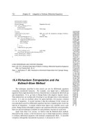
... Seinfeld, J. 19 71, Numerical Solution of Ordinary Differential Equations (New York: Academic Press). 16 .1 Runge-Kutta Method The formula for the Euler method is y n +1 = y n + hf(x n ,y n ) (16 .1. 1) whichadvances ... across the whole interval. Figure 16 .1. 2 illustrates the idea. In equations, k 1 = hf(x n ,y n ) k 2 =hf  x n + 1 2 h, y n + 1 2 k 1  y n +1 = y n + k 2 + O(h 3 ) (16 .1. 2) As indicated in the error ... conditions 707 710 Chapter 16 . Integration of Ordinary Differential Equations Sample page from NUMERICAL RECIPES IN C: THE ART OF SCIENTIFIC COMPUTING (ISBN 0-5 21- 4 310 8-5) Copyright (C) 19 88 -19 92 by...

Ngày tải lên: 15/12/2013, 04:15

Ngày tải lên: 08/04/2014, 12:24

Ngày tải lên: 08/04/2014, 12:25

Ngày tải lên: 20/06/2014, 21:20

Ngày tải lên: 22/06/2014, 02:20

Ngày tải lên: 22/06/2014, 21:20

... equation (19 .1. 20) is r n +1 j +1/ 2 − r n j +1/ 2 ∆t = s n +1/ 2 j +1 − s n +1/ 2 j ∆x s n +1/ 2 j − s n 1/ 2 j ∆t = v r n j +1/ 2 − r n j 1/ 2 ∆x (19 .1. 35) If you substitute equation (19 .1. 22) in equation (19 .1. 35), ... equation (19 .1. 15) so that it is in the form of equation (19 .1. 11) with a remainder term: u n +1 j − u n j ∆t = −v  u n j +1 − u n j 1 2∆x  + 1 2  u n j +1 − 2u n j + u n j 1 ∆t  (19 .1. 18) But ... time. where α ≡ v∆t ∆x (19 .1. 40) Then ξ =1 iα sin k∆x − α 2 (1 − cos k∆x) (19 .1. 41) so |ξ| 2 =1 α 2 (1 − α 2 ) (1 − cos k∆x) 2 (19 .1. 42) The stability criterion |ξ| 2 ≤ 1 is therefore α 2 ≤ 1, or v∆t ≤ ∆x...

Ngày tải lên: 07/11/2013, 19:15

... of Equations Sample page from NUMERICAL RECIPES IN C: THE ART OF SCIENTIFIC COMPUTING (ISBN 0-5 21- 4 310 8-5) Copyright (C) 19 88 -19 92 by Cambridge University Press.Programs Copyright (C) 19 88 -19 92 ... of Equations Sample page from NUMERICAL RECIPES IN C: THE ART OF SCIENTIFIC COMPUTING (ISBN 0-5 21- 4 310 8-5) Copyright (C) 19 88 -19 92 by Cambridge University Press.Programs Copyright (C) 19 88 -19 92 ... IN C: THE ART OF SCIENTIFIC COMPUTING (ISBN 0-5 21- 4 310 8-5) Copyright (C) 19 88 -19 92 by Cambridge University Press.Programs Copyright (C) 19 88 -19 92 by Numerical Recipes Software. Permission is...

Ngày tải lên: 07/11/2013, 19:15

... Seinfeld, J. 19 71, Numerical Solution of Ordinary Differential Equations (New York: Academic Press). 16 .1 Runge-Kutta Method The formula for the Euler method is y n +1 = y n + hf(x n ,y n ) (16 .1. 1) whichadvances ... across the whole interval. Figure 16 .1. 2 illustrates the idea. In equations, k 1 = hf(x n ,y n ) k 2 =hf  x n + 1 2 h, y n + 1 2 k 1  y n +1 = y n + k 2 + O(h 3 ) (16 .1. 2) As indicated in the error ... xh,hh,h6,*dym,*dyt,*yt; dym=vector (1, n); dyt=vector (1, n); 16 .1 Runge-Kutta Method 711 Sample page from NUMERICAL RECIPES IN C: THE ART OF SCIENTIFIC COMPUTING (ISBN 0-5 21- 4 310 8-5) Copyright (C) 19 88 -19 92 by Cambridge...

Ngày tải lên: 15/12/2013, 04:15

... slight generalization of (19 .2.8) leads to i  ψ n +1 j − ψ n j ∆t  = −  ψ n +1 j +1 − 2ψ n +1 j + ψ n +1 j 1 (∆x) 2  + V j ψ n +1 j (19 .2.27) for which ξ = 1 1+i  4∆t (∆x) 2 sin 2  k∆x 2  + V j ∆t  (19 .2.28) This ... is second-order accurate and unitary: e −iHt  1 − 1 2 iH∆t 1+ 1 2 iH∆t (19 .2.35) In other words,  1+ 1 2 iH∆t  ψ n +1 j =  1 − 1 2 iH∆t  ψ n j (19 .2.36) On replacing H by its finite-difference ... equation (19 .2 .19 ) write D j +1/ 2 = 1 2  D(u n j +1 )+D(u n j )  (19 .2.22) Implicit schemes are not as easy. The replacement (19 .2.22) with n → n +1leaves us with a nasty set of coupled nonlinear equations...

Ngày tải lên: 15/12/2013, 04:15

... is u n +1 j,l = 1 4 (u n j +1, l + u n j 1, l + u n j,l +1 + u n j,l 1 ) − ∆t 2∆ (F n j +1, l − F n j 1, l + F n j,l +1 − F n j,l 1 ) (19 .3.3) Note that as an abbreviated notation F j +1 and F j 1 refer ... is second-order accurate and unitary: e −iHt  1 − 1 2 iH∆t 1+ 1 2 iH∆t (19 .2.35) In other words,  1+ 1 2 iH∆t  ψ n +1 j =  1 − 1 2 iH∆t  ψ n j (19 .2.36) On replacing H by its finite-difference ... treated implicitly: u n +1/ 2 j,l = u n j,l + 1 2 α  δ 2 x u n +1/ 2 j,l + δ 2 y u n j,l  u n +1 j,l = u n +1/ 2 j,l + 1 2 α  δ 2 x u n +1/ 2 j,l + δ 2 y u n +1 j,l  (19 .3 .16 ) The advantage of this...

Ngày tải lên: 15/12/2013, 04:15

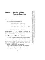
... Introduction A set of linear algebraic equations looks like this: a 11 x 1 + a 12 x 2 + a 13 x 3 + ···+a 1N x N =b 1 a 21 x 1 + a 22 x 2 + a 23 x 3 + ···+a 2N x N =b 2 a 31 x 1 + a 32 x 2 + a 33 x 3 + ···+a 3N x N =b 3 ··· ... ···+a 3N x N =b 3 ··· ··· a M1 x 1 +a M2 x 2 +a M3 x 3 +···+a MN x N = b M (2.0 .1) Here the N unknowns x j , j =1, 2, ,N are related by M equations. The coefficients a ij with i =1, 2, ,M and j =1, 2, ,N are known ... is the right-hand side written as a column vector, A =    a 11 a 12 a 1N a 21 a 22 a 2N ··· a M1 a M2 a MN    b =    b 1 b 2 ··· b M    (2.0.3) By convention, the first index on an...

Ngày tải lên: 15/12/2013, 04:15

... the three equations, we get u j−2 + T (1) · u j + u j+2 = g (1) j ∆ 2 (19 .4.32) This is an equation of the same form as (19 .4.29), with T (1) = 21 T 2 g (1) j =∆ 2 (g j 1 −T·g j +g j +1 ) (19 .4.33) After ... f l (19 .4 .17 ) The model equation (19 .0.3) becomes ∇ 2 u  = −∇ 2 u B + ρ (19 .4 .18 ) or, in finite-difference form, u  j +1, l + u  j 1, l + u  j,l +1 + u  j,l 1 − 4u  j,l = − (u B j +1, l + u B j 1, l + ... writing down three successive equations like (19 .4.29): u j−2 + T · u j 1 + u j = g j 1 ∆ 2 u j 1 + T · u j + u j +1 = g j ∆ 2 u j + T · u j +1 + u j+2 = g j +1 ∆ 2 (19 .4. 31) Matrix-multiplyingthe middle...

Ngày tải lên: 15/12/2013, 04:15

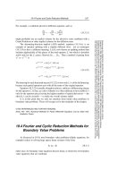
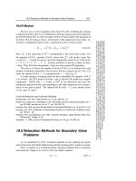
... In matrix notation, equations (19 .5.35) are (L x + r1) · u n +1/ 2 =(r1−L y )·u n −∆ 2 ρ (19 .5.36) (L y + r1) · u n +1 =(r1−L x )·u n +1/ 2 − ∆ 2 ρ (19 .5.37) where r ≡ 2∆ 2 ∆t (19 .5.38) The matrices ... equation (19 .5. 31) implicitly in two half-steps: u n +1/ 2 − u n ∆t/2 = − L x u n +1/ 2 + L y u n ∆ 2 − ρ u n +1 − u n +1/ 2 ∆t/2 = − L x u n +1/ 2 + L y u n +1 ∆ 2 − ρ (19 .5.35) (cf. equation 19 .3 .16 ). Here ... according to the following prescription: ω (0) =1 ω (1/ 2) =1/ (1 − ρ 2 Jacobi /2) ω (n +1/ 2) =1/ (1 − ρ 2 Jacobi ω (n) /4),n =1/ 2 ,1, , ∞ ω (∞) → ω optimal (19 .5.30) 19 .5 Relaxation Methods for Boundary Value...

Ngày tải lên: 15/12/2013, 04:15

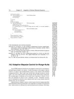
... a i b ij c i c ∗ i 1 37 378 2825 27648 2 1 5 1 5 0 0 3 3 10 3 40 9 40 250 6 21 18575 48384 4 3 5 3 10 − 9 10 6 5 12 5 594 13 525 55296 5 1 − 11 54 5 2 − 70 27 35 27 0 277 14 336 6 7 8 16 31 55296 17 5 512 575 13 824 44275 11 0592 253 4096 512 17 71 1 4 j ... -0.9,b43 =1. 2, b 51 = -11 .0/54.0, b52=2.5,b53 = -70.0/27.0,b54=35.0/27.0, b 61= 16 31. 0/55296.0,b62 =17 5.0/ 512 .0,b63=575.0 /13 824.0, b64=44275.0 /11 0592.0,b65=253.0/4096.0,c1=37.0/378.0, c3=250.0/6 21. 0,c4 =12 5.0/594.0,c6= 512 .0 /17 71. 0, dc5 ... y(x) z 1 = z 0 + hf(x, z 0 ) z m +1 = z m 1 +2hf(x + mh, z m ) for m =1, 2, ,n 1 y(x+H)≈y n ≡ 1 2 [z n +z n 1 +hf(x + H, z n )] (16 .3.2) 714 Chapter 16 . Integration of Ordinary Differential Equations Sample...

Ngày tải lên: 24/12/2013, 12:16

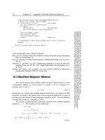
... for the method are z 0 ≡ y(x) z 1 = z 0 + hf(x, z 0 ) z m +1 = z m 1 +2hf(x + mh, z m ) for m =1, 2, ,n 1 y(x+H)≈y n ≡ 1 2 [z n +z n 1 +hf(x + H, z n )] (16 .3.2) 16 .3 Modified Midpoint Method 723 Sample ... 722 Chapter 16 . Integration of Ordinary Differential Equations Sample page from NUMERICAL RECIPES IN C: THE ART OF SCIENTIFIC COMPUTING (ISBN 0-5 21- 4 310 8-5) Copyright (C) 19 88 -19 92 by Cambridge ... FURTHER READING: Gear, C.W. 19 71, Numerical Initial Value Problems in Ordinary Differential Equations (Englewood Cliffs, NJ: Prentice-Hall). [1] Cash, J.R., and Karp, A.H. 19 90, ACM Transactions on...

Ngày tải lên: 24/12/2013, 12:16

... nseq[IMAXX +1] ={0,2,4,6,8 ,10 ,12 ,14 ,16 ,18 }; int reduct,exitflag=0; d=matrix (1, nv ,1, KMAXX); err=vector (1, KMAXX); x=vector (1, KMAXX); yerr=vector (1, nv); ysav=vector (1, nv); yseq=vector (1, nv); if (eps ... else { for (j =1; j<=nv;j++) c[j]=yest[j]; for (k1 =1; k1<iest;k1++) { delta =1. 0/(x[iest-k1]-xest); f1=xest*delta; f2=x[iest-k1]*delta; for (j =1; j<=nv;j++) { Propagate tableau 1 diagonal more. q=d[j][k1]; d[j][k1]=dy[j]; delta=c[j]-q; dy[j]=f1*delta; c[j]=f2*delta; yz[j] ... recurrence A 1 = n 1 +1 A k +1 = A k + n k +1 (16 .4.6) 730 Chapter 16 . Integration of Ordinary Differential Equations Sample page from NUMERICAL RECIPES IN C: THE ART OF SCIENTIFIC COMPUTING (ISBN 0-5 21- 4 310 8-5) Copyright...

Ngày tải lên: 24/12/2013, 12:16

... following set of equations [1] : u  = 998u + 19 98v v  = −999u − 19 99v (16 .6 .1) with boundary conditions u(0) = 1 v(0) = 0 (16 .6.2) By means of the transformation u =2y−zv=−y+z (16 .6.3) we find ... 734 Chapter 16 . Integration of Ordinary Differential Equations Sample page from NUMERICAL RECIPES IN C: THE ART OF SCIENTIFIC COMPUTING (ISBN 0-5 21- 4 310 8-5) Copyright (C) 19 88 -19 92 by Cambridge ... =2e −x −e 10 00x v = −e −x + e 10 00x (16 .6.4) If we integrated the system (16 .6 .1) with any of the methods given so far in this chapter, the presence of the e 10 00x term would require a stepsize h  1/ 1000...

Ngày tải lên: 24/12/2013, 12:16