ông a chết thì a b 283 2 141 5 trđ

Nonlinear Model Predictive Control: Theory and Algorithms (repost)

... 27 5 27 5 28 8 29 2 3 15 324 331 3 35 337 337 Appendix NMPC Software Supporting This Book A. 1 The MATLAB NMPC Routine A. 2 Additional MATLAB and MAPLE Routines A. 3 The C++ NMPC Software ... important topics beyond stability and performance, like feasibility, robustness, and numerical methods As a result, this book has become a mixture between a research monograph and an advanced textbook ... Teel, A. R.: Model predictive control: for want of a local control Lyapunov function, all is not lost IEEE Trans Automat Control 50 (5) , 54 6 55 8 (20 05) 12 Jadbabaie, A. , Hauser, J.: On the stability...

Báo cáo hóa học: "Research Article Neural Network Adaptive Control for Discrete-Time Nonlinear Nonnegative Dynamical Systems" ppt

Danh mục: Báo cáo khoa học

... partitioned as K note that ⎡ BK T ⎣ BK1 T AT 21 A1 2 A A11 BK2 T AT 22 ⎤ ⎦ 2. 7 Assume that A BK is nonnegative and asymptotically stable, and suppose that, ad absurdum, A2 2 is not asymptotically stable ... that A2 2 is asymptotically stable Then taking K1 B −1 As − A1 1 and K2 B −1 A1 2 , where As is nonnegative and asymptotically stable, it follows that spec A BK ∩ C1 spec As ∪ spec A2 2 ∩ C1 Ø, and ... in 2. 4 be partitioned as A A11 A1 2 , A2 1 A2 2 2.6 where A1 1 ∈ Rm×m , A1 2 ∈ Rm× n−m , A2 1 ∈ R n−m ×m , and A2 2 ∈ R n−m × n−m are nonnegative matrices 4 Advances in Diﬀerence Equations Theorem 2. 4...

ON STABILITY ZONES FOR DISCRETE-TIME PERIODIC LINEAR HAMILTONIAN SYSTEMS ˘ VLADIMIR RASVAN Received potx

Danh mục: Báo cáo khoa học

... Halanay and V Ionescu, Time-Varying Discrete Linear Systems, Operator Theory: Advances and Applications, vol 68, Birkh¨ user Verlag, Basel, 1994 a [14] A Halanay and Vl R˘ svan, Stability and boundary ... Matematicheski˘ Sbornik 16 (1891/1893), 5 82 59 1 (Russian) ı Vladimir R˘ svan: Department of Automatic Control, University of Craiova, Street A I Cuza no 13, a RO -20 058 5, Craiova, Romania E-mail ... the American Mathematical Society 24 6 (1978), 1–30 [17] W Kratz, Quadratic Functionals in Variational Analysis and Control Theory, Mathematical Topics, vol 6, Akademie Verlag, Berlin, 19 95 [18]...

Báo cáo sinh học: " Heritability of longevity in Large White and Landrace sows using continuous time and grouped data models" ppsx

Danh mục: Báo cáo khoa học

... 10th farrowing Only sows born after 19 95 were included in the evaluation and age at first farrowing between 25 0 and 55 0 days was required The analysis was carried out using a proportional hazards ... life was analyzed for 123 19 Large White sows originating from 838 boars and 4348 dams and for 9833 Landrace sows originating from 457 boars and 22 36 dams Overall survival for both populations ... http://www.gsejournal.org/content/ 42/ 1/13 Page of 13 Table 1: Statistical overview Large White a Landrace b mean std mean std Parity 4.14 2. 87 4.70 3.03 non-censored 4.31 2. 94 4.81 3.08 censored 3 .55 2. 52 4.09 2. 62 LPL at last...

Adaptive control and neural network control of nonlinear discrete time systems

Danh mục: Cao đẳng - Đại học

... backstepping But these approaches are not applicable to nonaﬃne systems, especially feedback linearization based methods, which greatly depends the a ne appearance of control variables As a matter of fact, ... Mr Aswin Thomas Abraham, Dr Brice Rebsamen, Dr Bingbing Liu, Dr Qinghua Xia, Ms Bahareh Ghotbi, Mr Dong Huang and many others that have been part of the team, for the stressful but exciting time ... approximation ability has been developed based on the Stone-Weierstrass theorem, which states that a universal approximator can approximate, to an arbitrary degree of accuracy, any real continuous...

Changes of temperature data for energy studies over time and their impact on energy consumption and CO2 emissions. The case of Athens and Thessaloniki – Greece

Danh mục: Môi trường

... Base Temperature 20 22 24 26 20 22 24 26 20 22 24 26 20 22 24 26 20 22 24 26 1983 – 19 92 114 74 43 23 186 1 32 87 53 174 121 79 47 84 51 28 13 55 8 378 23 7 136 Period 1993 – 20 02 137 92 56 30 20 5 ... 20 13, pp .59 - 72 65 Table Monthly cooling degree days to various temperature bases - Athens Greece Month Jun Jul Aug Sep Total Base Temperature 20 22 24 26 20 22 24 26 20 22 24 26 20 22 24 26 20 ... 20 02 74 42 22 10 196 143 96 59 33 327 26 6 20 7 151 1 02 3 62 300 23 9 180 1 25 28 7 23 2 179 130 86 24 9 191 138 91 55 130 85 49 24 10 1 6 25 1 25 9 930 6 45 4 15 1983 – 20 02 82 48 25 11 20 6 151 1 02 63 35 340...

Tài liệu ADVANCES IN DISCRETE TIME SYSTEMS docx

Danh mục: Kỹ thuật lập trình

... Delays Descriptor Systems with Delays Jun Yoneyama, Yuzu Uchida and Ryutaro Takada Jun Yoneyama, Yuzu Uchida and Ryutaro Takada Additional information available at at end of of chapter Additional ... 0 .55 71 − 0 .28 86 − 1.99 92 p1 = − 0 .29 51 , p2 = 0 .20 65 X1>0 0 .55 53 − 0 .28 92 − 2. 0113 p1 = − 0.1 653 , p2 = 0.0761 X2>0 0 .54 96 − 0 .29 03 − 2. 023 7 p1 ,2 = − 0.0 451 ± j0.18 62 X3>0 0 .53 98 − 0 .29 18 − 2. 0363 ... Xia, Li Dai, Magdi Mahmoud, Meng-Yin Fu, Mario Alberto Jordan, Jorge Bustamante, Carlos Berger, Atsue Ishii, Takashi Nakamura, Yuko Ohno, Satoko Kasahara, Junmin Li, Jiangrong Li, Zhile Xia, Saïd...

Discrete time control systems pptx

Danh mục: Điện - Điện tử

...

Discrete Time Systems Part 1 pdf

Danh mục: Kĩ thuật Viễn thông

... may not easily be calculated for state models with nonlinear disturbance noise (Arulampalam et al., 20 02; Ristic et al., 20 04) The Demirba¸ s estimation approaches are more general than grid-based ... must be satisﬁed by an approximate discrete random variable with n possible values of an absolutely continuous random variable is given (Demirba¸ , 19 82; 1984; 20 10); ﬁnally, the s approximate ... discrete random variables of a Gaussian random variable are tabulated Let w be an m-dimensional random vector An approximate discrete random vector with n possible values of w, denoted by wd ,...

Discrete Time Systems Part 2 potx

Danh mục: Kĩ thuật Viễn thông

... 0.1 72 0 .29 8 0.384 0 .50 0 0. 656 0.187 0.3 05 0.4 52 0.6 02 0. 754 0. 826 1.4 75 1.863 2. 5 52 3.137 1. 024 1.743 2. 454 3.306 4 .20 3 0.1 85 0.310 0.4 05 0 .55 0 0.691 0 .20 0 0.340 0.471 0. 621 0.776 Table Comparison ... industrial tasks, military commands, mobile robot navigation, multi-target tracking, and aircraft navigation (see (hall, 19 92, Bar-Shalom, 1990, Bar-Shalom & Li, 19 95, Zhu, 20 02, Ren & Key, 1989) and ... Balakrishnan, V (1994) Linear matrix inequalities in system and control theory, SIAM Studies in Applied Mathematics, Philadelphia, USA Cherrier, E., Boutayeb, M & Ragot, J (20 05) Observers based...

Discrete Time Systems Part 3 ppt

Danh mục: Kĩ thuật Viễn thông

... R J Patton (1998) and Sawada & Tanikawa (20 02) and the book Chen & Patton (1999) Their algorithm recently has been modiﬁed by the author in Tanikawa (20 06) (see Tanikawa & Sawada (20 03) also) ... research papers have been published based on the disturbance decoupling principle Pioneering works were done by Darouach et al (Darouach; Zasadzinski; Bassang & Nowakowski (19 95) and Darouach; Zasadzinski ... the mean-square error in an appropriate class of linear ﬁlters (see e.g., Kailath (1974), Kailath (1976), Kalman (1960), Kalman (1963) and Katayama (20 00)) But we note that the Kalman ﬁlter can...

Discrete Time Systems Part 4 pptx

Danh mục: Kĩ thuật Viễn thông

... Transactions on Automatic Control 51 (8): 1 354 –1 358 Kalman, R E (1960) A New Approach to Linear Filtering and Prediction Problems, Transactions of the ASME 82 (1): 35- 45 Sayed, A H (20 01) A framework ... n×n be a positive-semideﬁnite matrix and A ∈ R n×n be diagonalizable, i.e., it can be written as A = VDV −1 , ( 155 ) max eig( A) 2 b < 1, ( 156 ) with D diagonal If then, ⎛ ⎞ ∞ Tr ⎝ ∑ b j A j XA j ⎠ ... more material to buy, a heavier product) b) Some states are impossible to be physically measured because they are a mathematically useful representation of the system, such as, the attitude parameterization...

Discrete Time Systems Part 5 potx

Danh mục: Kĩ thuật Viễn thông

... Shaked (1997); Gershon et al (20 0 4a) ; Gershon et al (20 0 4b) ; Nakura (20 0 8a) ; Nakura (20 0 8b) ; Nakura (20 08c); Nakura (20 08d); Nakura (20 08e); Nakura (20 09); Nakura (20 10); Sawada (20 08); Shaked ... As is a stable polynomial The characteristic polynomial of AS is calculated as the next equation From Eq. (26 ), zE − As can be shown as zE − A + BE2C G1E2C zE − As = −G2C BH zI − F1 + G1 H BH G1 ... available, d( k ), d0 ( k ) are bounded disturbances, ym ( k ) is the model output The basic assumptions are as follows: Assume that (C , A , B) is controllable and observable, i.e ⎡ zE − A ⎤...

Discrete Time Systems Part 6 pptx

Danh mục: Kĩ thuật Viễn thông

... − T − γ 2 AT X∞ B1 U 1B1 X∞ B2 U 1B2 U A + γ 2 ATU B2 U 1B2 X∞ B1 U 1B1 X∞ B2 U 1B2 U A) − − T − T − T = ( A − B2 U 1BTU A) T X∞ ( A − B2 U 1B2 U A) + (C − D12U 1B2 U A) T (C − D12U 1B2 U A) − T − T ... X∞ B2 U 1B2 U A + ATU B2 U 1B2 X∞ B2 U 1B2 U A) T − − T − − T + (C C + ATU B2 U 1U 1B2 U A) + ATU B2 U RU 1B2 U A + Q − T − T − T + (γ 2 AT X∞ B1 U 1B1 X∞ A − γ 2 ATU B2 U 1B2 X∞ B1 U1 1B1 X∞ A − T − ... ) A − T − T − AT ( X∞ + γ 2 X∞ B1 U 1B1 X∞ )B2 U 1B2 U A T − T − − T + ATU B2 U 1[ R + I + B2 ( X∞ + γ 2 X∞ B1 U1 1B1 X∞ )B2 ]U 1B2 U A − T − T − T − T = ( AT X∞ A − ATU B2 U 1B2 X∞ A − AT X∞ B2 U...

Discrete Time Systems Part 7 ppt

Danh mục: Kĩ thuật Viễn thông

... ATU B2 U 1B2 U A This implies that (21 ) can be rewritten as − T T − T T AT X∞ A − X∞ + γ 2 AT X∞ B1 U 1B1 X∞ A + C C + Qδ − ATU 3B2 U 1B2 U A + ρ EK EK = ( 25 ) Thus, it follows from (24 ) and ( 25 ) ... T T T T T = AT X∞ A − X∞ + γ 2 AT X∞ B1 U1 1B1 X∞ A + C C + Q + F∞ B2 U A + ATU B2 F∞ + F∞ U F∞ (22 ) − T − T T = AT X∞ A − X∞ + γ 2 AT X∞ B1 U1 1B1 X∞ A + C C + Q − ATU B2 U 1B2 U A + ΔN T T where, ... Problems − T ˆ ˆ ˆ ˆ ˆ Note that A − B( BT X∞ B + R )−1 BT X∞ A = AF∞ + γ 2 B1 U 1B1 X∞ AF∞ is stable and ΔF( k ) is an − T admissible uncertainty, we get that AF + γ 2 BF U1 1BF X∞ AF is stable...

Discrete Time Systems Part 8 pot

Danh mục: Kĩ thuật Viễn thông

... uncertainty can be dealt with by feedback?, IEEE Transactions on Automatic Control 45( 12) : 22 03 22 17 22 8 Discrete Time Systems Xu, J.-X & Huang, D (20 09) Discrete-time adaptive control for a class ... C (20 01) Robust adaptive control of nonlinear discrete-time systems by backstepping without overparameterization, Automatica 37(4): 55 1 – 55 8 Zhang, Y X & Guo, L (20 02) A limit to the capability ... Control and Automation, Hangzhou China, June 20 04, Vol 2, pp 1 52 1 -1 52 4 D Zhang, Z Wang, and S Hu Robust satisfactory fault-tolerant control of uncertain linear discrete-time systems: an LMI approach,...

Discrete Time Systems Part 9 ppt

Danh mục: Kĩ thuật Viễn thông

... following basic problem: Is it possible for all of the agents to achieve a global goal based on the local information and local control? Here the global goal may refer to global stability, synchronization, ... uncertainty can be dealt with by feedback?, IEEE Transactions on Automatic Control 45( 12) : 22 03 22 17 Yang, C., Dai, S.-L., Ge, S S & Lee, T H (20 09) Adaptive asymptotic tracking control of a class ... exogenous perturbations 3.3 Sampled-data model Usually, sampled-data behavior can be modelled by n-steps-ahead predictors (Jordán & Bustamante, 20 0 9a) Accordingly, we attempt now to translate the continuous...

Discrete Time Systems Part 10 pdf

Danh mục: Kĩ thuật Viễn thông

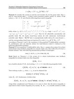
... together by means of a visualization program (see a photogram in Fig 2) The units for the path run away are in meters Basically the vehicle turns around a planar path At a certain coordinate A it leaves ... Perturbed Measures for Complex Dynamics - Case Study: Unmanned Underwater Vehicles 27 5 and the mass variations are MbΔ+ = diag(10, 10, 10, 0. 6 25 0, 4 .22 50 , 3.6) (86) MbΔ− = diag (20 , 20 , 20 , 1 . 25 , ... the body matrix Mb and the additive matrix Ma given by Mb = Mbn + δ(t − t A ) MbΔ+ − δ(t − t B ) MbΔ− (83) Ma = Man + δ(t − t A ) MaΔ+ − δ(t − t B ) MaΔ− , (84) where Mbn and Man are nominal values...

Discrete Time Systems Part 11 potx

Danh mục: Kĩ thuật Viễn thông

... R p×n , a scalar variable θ ∈]0, 1] and for a given μ = 2 such that ⎡ ˜ T ˜ T Am F11 Am F 12 P11i − F11 − F11 P12i − F 12 − Λ T F 22 T ˜ ⎢ P22i − F 22 − F 22 ( Ai F 22 + Bi W )Λ Ai F 22 + Bi W ⎢ ⎢ ... with A1 and ˜ ˜ ˜ ˜ ˜ Ad1 given by ( 35) and A2 = 1.1 A1 and Ad2 = 1.1 Ad1 In this case the conditions of Boukas (20 06) are no longer applicable and those from Liu et al (20 06) are not directly applied, ... −0. 124 72 ⎥ ⎥ ⎢ B = B0 = ⎢ 0 .29 469 0.31 52 8 1.16 420 −0 .29 922 0 .23 883 ⎥ , ⎥ ⎢ ⎣ −0 .20 191 0.19739 0.41686 0.6 655 1 0.11366 ⎦ −0.118 35 0.1 628 7 0 .20 378 0 .23 261 0.36 52 5 ⎡ (58 ) (59 ) and C = D = I5 , Cd = 0,...

Discrete Time Systems Part 12 ppt

Danh mục: Kĩ thuật Viễn thông

... ( A2 1 ) T P 22 A2 2 (4. 12) i i ¯i i ¯i ¯i ¯i ¯i ¯i ¯i ¯i 22 = ( A1 2 ) T P11 A1 2 + ( A2 2 ) T ( P 12 ) T A1 2 + ( A1 2 ) T P 12 A2 2 + ( A2 2 ) T P 22 A2 2 ¯i At this point, we declare A2 2 is nonsingular ... 0. 12 ≤ 22 ≤ 0 .24 and b 0. 12 ≤ b ≤ 0 .24 , 0. 12 ≤ ⊗ 12 ≤ 0 .24 , 0. 12 ≤ b ≤ 0.18, 0 .24 ≤ b ≤ 0.30 11 21 22 Equation ( 15) and ( 25 ) give ⎡ -0 .24 0. 12 ⎤ ⎡ 0 .24 0 .24 ⎤ ⎡0. 12 0. 12 ⎤ ⎡0 .24 0 .24 ⎤ , A2 = ... described by (13), where ⎡ a AI ( ⊗ ) = ⎢ 11 a ⎢ 21 ⎣ a b ⎡⊗11 ⊗ 12 ⎤ ⎥ , BI ( ⊗ ) = ⎢ b a 22 ⎥ ⎢ 21 ⎦ ⎣ b ⊗ 12 ⎤ ⎥, b ⎥ 22 ⎦ a a a a with -0 .24 ≤ ⊗11 ≤ 0 .24 , 0. 12 ≤ ⊗ 12 ≤ 0 .24 , -0. 12 ≤ 21 ≤ 0. 12, ...

Xem thêm

Tìm thêm: hệ việt nam nhật bản và sức hấp dẫn của tiếng nhật tại việt nam xác định các mục tiêu của chương trình xác định các nguyên tắc biên soạn khảo sát các chuẩn giảng dạy tiếng nhật từ góc độ lí thuyết và thực tiễn khảo sát chương trình đào tạo của các đơn vị đào tạo tại nhật bản khảo sát chương trình đào tạo gắn với các giáo trình cụ thể điều tra đối với đối tượng giảng viên và đối tượng quản lí điều tra với đối tượng sinh viên học tiếng nhật không chuyên ngữ1 xác định mức độ đáp ứng về văn hoá và chuyên môn trong ct mở máy động cơ lồng sóc mở máy động cơ rôto dây quấn các đặc tính của động cơ điện không đồng bộ hệ số công suất cosp fi p2 đặc tuyến mômen quay m fi p2 đặc tuyến tốc độ rôto n fi p2 động cơ điện không đồng bộ một pha thông tin liên lạc và các dịch vụ từ bảng 3 1 ta thấy ngoài hai thành phần chủ yếu và chiếm tỷ lệ cao nhất là tinh bột và cacbonhydrat trong hạt gạo tẻ còn chứa đường cellulose hemicellulose chỉ tiêu chất lượng theo chất lượng phẩm chất sản phẩm khô từ gạo của bộ y tế năm 2008 chỉ tiêu chất lượng 9 tr 25