Electromagnetic Waves and Antennas combined - Chapter 1 pps
Electromagnetic Waves and Antennas combined - Chapter 1 pps
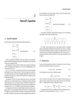
... that: σ = Ne 2 mγ = ( 8.4 × 10 28 ) (1. 6 × 10 19 ) 2 (9 .1 × 10 − 31 )(4 .1 × 10 13 ) = 5.8 × 10 7 Siemens/m where we used e = 1. 6 × 10 19 , m = 9 .1 × 10 − 31 , γ = 4 .1 × 10 13 . The plasma frequency of ... formula [14 7], where λ and λ i are in units of μm: n 2 = 1 + 0.69 616 63 λ 2 λ 2 −(0.0684043) 2 + 0.4079426 λ 2 λ 2 −(0 .11 62 414 ) 2 + 0.8974794 λ 2...
Ngày tải lên: 13/08/2014, 02:20
Electromagnetic Waves and Antennas combined - Chapter 2 potx
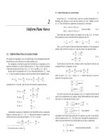
... application of Eq. (2 .11 .13 ) to S a and S b gives: f a = f 1 −β a 1 +β a ,f b = f 1 −β b 1 +β b ⇒ f b = f a 1 −β b 1 +β b · 1 +β a 1 −β a (2 .11 .14 ) where β a = v a /c and β b = v b /c. This ... 59 (1 −jτ) 1/ 2 = ⎧ ⎪ ⎨ ⎪ ⎩ 1 −j τ 2 , if τ 1 e −jπ/4 τ 1/ 2 = (1 − j) τ 2 , if τ 1 (2.6.29) (1 −jτ) 1/ 2 = ⎧ ⎪ ⎪ ⎨ ⎪ ⎪ ⎩ 1 +j τ 2 , if τ 1 e j...
Ngày tải lên: 13/08/2014, 02:20
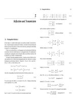
Electromagnetic Waves and Antennas combined - Chapter 3 ppt
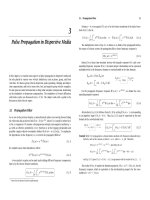
... vac 0 1 3 4 0 1 z/a t =0 0 1 3 4 0 1 z/a t =40 0 1 3 4 0 1 z/a t =12 0 0 1 3 4 0 1 z/a t =18 0 0 1 3 4 0 1 z/a t =220 0 1 3 4 0 1 z/a t =230 0 1 3 4 0 1 z/a t =240 0 1 3 4 0 1 z/a t =250 0 1 3 4 0 1 z/a t ... 3 4 0 1 z/a t = 12 0 0 1 3 4 0 1 z/a t =−50 vac abs vac gain vac 0 1 3 4 0 1 z/a t =0 0 1 3 4 0 1 z/a t =40 0 1 3 4 0 1 z/a t =12 0...
Ngày tải lên: 13/08/2014, 02:20
Electromagnetic Waves and Antennas combined - Chapter 4 pdf
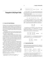
... (4.7.9) n 3 n 1 cos 2 θ + n 1 n 3 sin 2 θ = n 1 n 3 N 2 (4.7 .10 ) n 2 1 n 2 3 sin 2 θ + n 2 3 n 2 1 cos 2 θ = n 2 1 +n 2 3 −N 2 N 2 (4.7 .11 ) sin 2 θ = 1 − n 2 1 N 2 1 − n 2 1 n 2 3 , cos 2 θ = 1 − n 2 3 N 2 1 ... have a 1 = 1 and a 2 = 0, correspond- ing to α 1 = 0 and α 2 =∞. Typical values of the attenuations for commercially available polaroids are of t...
Ngày tải lên: 13/08/2014, 02:20
Electromagnetic Waves and Antennas combined - Chapter 5 ppt
... (5.4.9): E 1 H 1 = cos k 1 l 1 jη 1 sin k 1 l 1 jη 1 1 sin k 1 l 1 cos k 1 l 1 E 2 H 2 = cos k 1 l 1 jη 1 sin k 1 l 1 jη 1 1 sin k 1 l 1 cos k 1 l 1 cos k 2 l 2 jη 2 sin k 2 l 2 jη 1 2 sin ... Γ 1 and denoting z 1 = e 2jk 1 l 1 , z 2 = e 2jk 2 l 2 ,we eventually find: Γ 1 = ρ 1 +ρ 2 z 1 1 +ρ 1 ρ 2 ρ 3 z 1 2 +ρ 3...
Ngày tải lên: 13/08/2014, 02:20
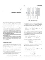
Electromagnetic Waves and Antennas combined - Chapter 6 potx
... Structures r= -0 .10 00 -0 .2000 -0 .4000 0.5000 A= 1. 0000 1. 0000 1. 0000 1. 0000 -0 .10 00 -0 .12 00 -0 .2000 0 -0 .0640 -0 .10 00 0 0 -0 .0500000 B= -0 .10 00 -0 .2000 -0 .4000 0.5000 -0 .18 80 -0 .3600 0.5000 0 -0 .3500 0.5000 ... 1, we have A 2 (z)= 1 and B 2 (z)= ρ 2 . Then, Eq. (6.6 .19 ) gives: A 1 (z) B 1 (z) = 1 ρ 1...
Ngày tải lên: 13/08/2014, 02:20
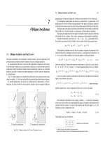
Electromagnetic Waves and Antennas combined - Chapter 7 potx
... ε 2r >ε 1 , we have ε 1 +ε 2 = √ ε 1 −ε 2r = j √ ε 2r −ε 1 , and ε 1 ε 2 = √ −ε 1 ε 2r = j √ ε 1 ε 2r . Then, Eqs. (7 .11 .5) read k x = k 0 ε 1 ε 2r ε 2r −ε 1 ,k z1 =−j k 0 ε 1 √ ε 2r −ε 1 ,k z2 =−j k 0 ε 2r √ ε 2r −ε 1 (7 .11 .7) 7 .11 . ... +cos 2 θ = n 2 1 + cos θ −β 1 −β cos θ 2 , or, n cos θ t = (n 2 1) (1 −β cos θ) 2 +(cos θ −β...
Ngày tải lên: 13/08/2014, 02:20

Electromagnetic Waves and Antennas combined - Chapter 8 pdf
... 1. 63, 1. 63] (b) n = [1. 54, 1. 54, 1. 63], n = [1. 5, 1. 5, 1. 5] (c) n = [1. 8, 1. 8, 1. 5], n = [1. 5, 1. 5, 1. 5] (d) n = [1. 8, 1. 8, 1. 5], n = [1. 56, 1. 56, 1. 56] 8 .11 . Brewster and Critical Angles ... n L = [1. 57, 1. 57, 1. 57]. The angle of incidence was θ a = 0 o . The typical MATLAB code was: LH = 0.25; LL = 0.25; na = [1; 1; 1] ; nb = [1; 1; 1] ;...
Ngày tải lên: 13/08/2014, 02:20

Electromagnetic Waves and Antennas combined - Chapter 9 potx
... 6.56 8.20 12 .50 X 250 kW 0 .11 0 WR-62 0.622 0. 311 9.49 11 .90 18 .00 Ku 14 0 kW 0 .17 6 WR-42 0.42 0 .17 14 .05 17 .60 26.70 K 50 kW 0.370 WR-28 0.28 0 .14 21 .08 26.40 40.00 Ka 27 kW 0.583 WR -1 5 0 .14 8 0.074 ... 0 (9 .1. 4) 9 .11 . Dielectric Slab Waveguides 389 1 k c H 1 cos k c a = 1 α c H 2 e −α c a and 1 k c H 1 cos k c a =− 1 α c H 3 e −α c a (9 .11 .10 ) Eqs....
Ngày tải lên: 13/08/2014, 02:20

Electromagnetic Waves and Antennas combined - Chapter 10 pdf
... AWG a Z RG-6/U 18 0. 512 75 RG-8/U 11 1. 150 50 RG -1 1 /U 14 0. 815 75 RG-58/U 20 0 .406 50 RG-59/U 22 0.322 75 RG -1 7 4/U 26 0.203 50 RG- 213 /U 13 0 . 915 50 The most commonly used cables are 5 0- ones, ... V L (t) 1 0 1 +2.25[0.4 1 ]= 1. 90 1. 5 1 +2.25[0.4 1 +0.4 2 ]= 2.26 1. 5 [1 +0.4 1 ]= 2 .10 1 +2.25[0.4 1 +0.4 2 +0.4 3 ]= 2.40 1. 5( [1 +0.4 1 +0.4 2 ]...
Ngày tải lên: 13/08/2014, 02:20
- routing protocols and concepts answers chapter 1
- ccna exploration routing protocols and concepts answers chapter 1
- ccna routing protocols and concepts answers chapter 1
- cisco routing protocols and concepts answers chapter 1
- think and grow rich chapter 1 review
- dr jekyll and mr hyde chapter 1 notes
- dr jekyll and mr hyde chapter 1 synopsis
- dr jekyll and mr hyde chapter 1 answers
- dr jekyll and mr hyde chapter 1 questions